


Analysis: 20251107
!pip install nucleus-cdk==0.5.0rc2 | tail -n2Requirement already satisfied: asttokens in /opt/homebrew/anaconda3/lib/python3.12/site-packages (from stack-data->ipython>=6.1.0->ipywidgets==8.*->jupyter-bokeh<5.0.0,>=4.0.5->nucleus-cdk==0.5.0rc2) (2.0.5)
Requirement already satisfied: pure-eval in /opt/homebrew/anaconda3/lib/python3.12/site-packages (from stack-data->ipython>=6.1.0->ipywidgets==8.*->jupyter-bokeh<5.0.0,>=4.0.5->nucleus-cdk==0.5.0rc2) (0.2.2)
import pandas as pd
import matplotlib.pyplot as plt
import seaborn as sns

from cdk.analysis.cytosol import platereader as pr

# Initialize plotting
pr.plot_setup()
Load the data
Provide a CSV file containing the data, and a platemap. This function returns both the data with the plate map mapped to it, and the platemap by itself, which is useful for certain tasks.
data_file = "./20251107-cytation3-pure-timecourse-gfp-MgSweep-biotek-cdk.txt"
platemap_file = "./20251107-NucleusPURE-deGFP-MgSweep-platemap.csv"

data, platemap = pr.load_platereader_data(data_file, platemap_file)
Basic Analysis
Curves
Curves of RFU over time, by named sample.
K=pr.plot_curves(data)
K.savefig('Kinetics')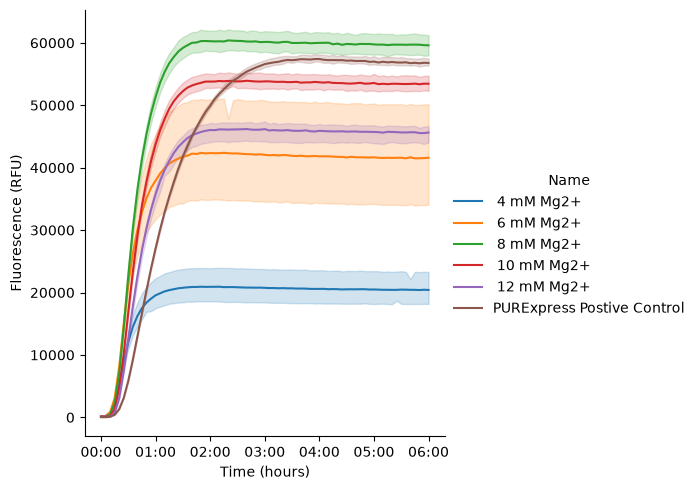
K=pr.plot_curves(data, units="Well", estimator=None)
K.axes.flatten()[0].axvline(pd.to_timedelta("04:00:00"), c="red", ls="--")
K.savefig('Kinetics2')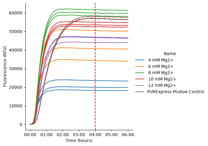
Steady state
Bar graph of steady-state endpoint of each sample. Steady state is calculated as the maximum fluorescence value over a 3-sample rolling average on the data.
There’s something weird going on with solving the kinetics. In the meantime, pick an appropriate-looking time for which to calculate steady state and use that. Here we chose four hours.
g = sns.catplot(
    data=data[data["Time"] == "04:00:00"],
    x="Name",
    y="Data",
    kind="bar"
)

g.set_xticklabels(rotation=90)
g.savefig('Steadystate')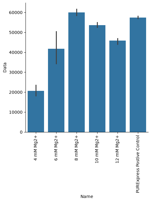
S= pr.plot_steadystate(data)
S.savefig('endpoint')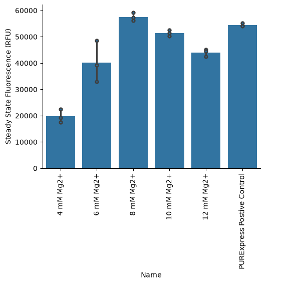
Kinetics
These functions calculate key kinetic parameters of the time series.
data["Read"].unique()array(['GFP-F-G35'], dtype=object)pr.kinetic_analysis(data, group_by=["Well"])Loading...
pr.plot_kinetics(data, group_by=["Well"])(<seaborn.axisgrid.FacetGrid at 0x13e9fa0d0>,
Velocity Lag \
Time Data Max Time
Well
B10 0 days 00:27:39.127690260 9192.42 35229.55 0 days 00:11:59.782011727
B12 0 days 00:27:43.051249782 10138.37 37157.67 0 days 00:11:20.801088528
B14 0 days 00:28:33.766010655 11837.93 43980.30 0 days 00:12:24.773821614
D10 0 days 00:29:23.447422773 17293.27 60560.09 0 days 00:12:15.447260347
D12 0 days 00:30:46.405018101 20630.07 66660.31 0 days 00:12:12.274964506
D14 0 days 00:31:27.283855339 25544.05 80829.33 0 days 00:12:29.595493450
F10 0 days 00:35:38.492638641 30160.54 86897.15 0 days 00:14:48.993116802
F12 0 days 00:35:28.883392526 31165.89 89568.65 0 days 00:14:36.244064184
F14 0 days 00:35:51.285870106 29554.62 83478.07 0 days 00:14:36.739825245
H10 0 days 00:38:28.682264936 27636.99 74344.32 0 days 00:16:10.406742063
H12 0 days 00:38:40.346870683 27046.79 71270.89 0 days 00:15:54.172648990
H14 0 days 00:39:02.188332878 26441.34 69933.30 0 days 00:16:21.051154290
J10 0 days 00:40:58.037015780 22324.78 54560.20 0 days 00:16:24.999916868
J12 0 days 00:40:51.829055425 23732.15 59092.05 0 days 00:16:46.021268027
J14 0 days 00:42:55.673906 23399.68 58266.42 0 days 00:18:49.920955700
L10 0 days 01:00:17.655535396 28572.32 39050.91 0 days 00:16:23.649294802
L12 0 days 00:59:57.207575047 28478.50 38879.07 0 days 00:16:00.246316310
L14 0 days 00:59:31.582831689 29050.87 39722.75 0 days 00:15:38.756388326
Steady State \
Data Time Data
Well
B10 1946.03 0 days 00:50:42.050705272 17465.60
B12 1782.80 0 days 00:51:49.139079674 19262.90
B14 2522.66 0 days 00:52:20.335195650 22492.07
D10 3403.54 0 days 00:54:36.889296055 32857.22
D12 3545.99 0 days 00:58:06.648996784 39197.14
D14 4446.65 0 days 00:59:22.210834282 48533.70
F10 5516.14 0 days 01:06:18.030185974 57305.03
F12 5406.09 0 days 01:06:13.043424358 59215.20
F14 5027.84 0 days 01:07:07.697397565 56153.78
H10 5017.56 0 days 01:11:18.917570763 52510.29
H12 4517.48 0 days 01:12:11.655185018 51388.91
H14 4792.55 0 days 01:12:26.081013898 50238.54
J10 3530.28 0 days 01:17:06.670940528 42417.08
J12 4032.95 0 days 01:16:20.375457596 45091.08
J14 5554.69 0 days 01:18:24.139576551 44459.39
L10 2759.44 0 days 02:04:55.490857903 54287.41
L12 2637.79 0 days 02:04:39.393333368 54109.15
L14 2600.60 0 days 02:04:07.681233284 55196.64
Fit
params R^2 drift good_fit
Well
B10 [18384.84651683236, 7.664909911789614, 0.46086... 1.00 42.33 True
B12 [20276.739358771836, 7.330108245084094, 0.4619... 0.99 109.15 True
B14 [23675.86813093157, 7.43040045761027, 0.476046... 0.99 51.71 True
D10 [34586.54334497583, 7.003889949217267, 0.48984... 0.99 124.11 True
D12 [41260.144555549006, 6.462441236034682, 0.5128... 0.99 236.75 True
D14 [51088.10700330671, 6.328622356833956, 0.52424... 0.99 283.71 True
F10 [60321.081181049594, 5.762307130054482, 0.5940... 1.00 291.03 True
F12 [62331.78504867434, 5.747863602961548, 0.59135... 1.00 351.60 True
F14 [59109.24325181486, 5.649070137273777, 0.59757... 1.00 350.59 True
H10 [55273.988141030204, 5.380058053806774, 0.6413... 1.00 289.88 True
H12 [54093.58486242694, 5.270191670492156, 0.64454... 1.00 336.64 True
H14 [52882.676262446716, 5.289694615579528, 0.6506... 1.00 266.38 True
J10 [44649.55280169389, 4.88786060387154, 0.682788... 1.00 312.95 True
J12 [47464.299550272786, 4.979915079217008, 0.6810... 1.00 284.05 True
J14 [46799.35977483207, 4.980103964867012, 0.71546... 0.99 -76.24 True
L10 [57144.63702325388, 2.7334787177483686, 1.0049... 1.00 818.32 True
L12 [56956.998924788815, 2.7304155403390835, 0.999... 1.00 859.42 True
L14 [58101.73071357878, 2.7347036186291556, 0.9921... 1.00 901.82 True )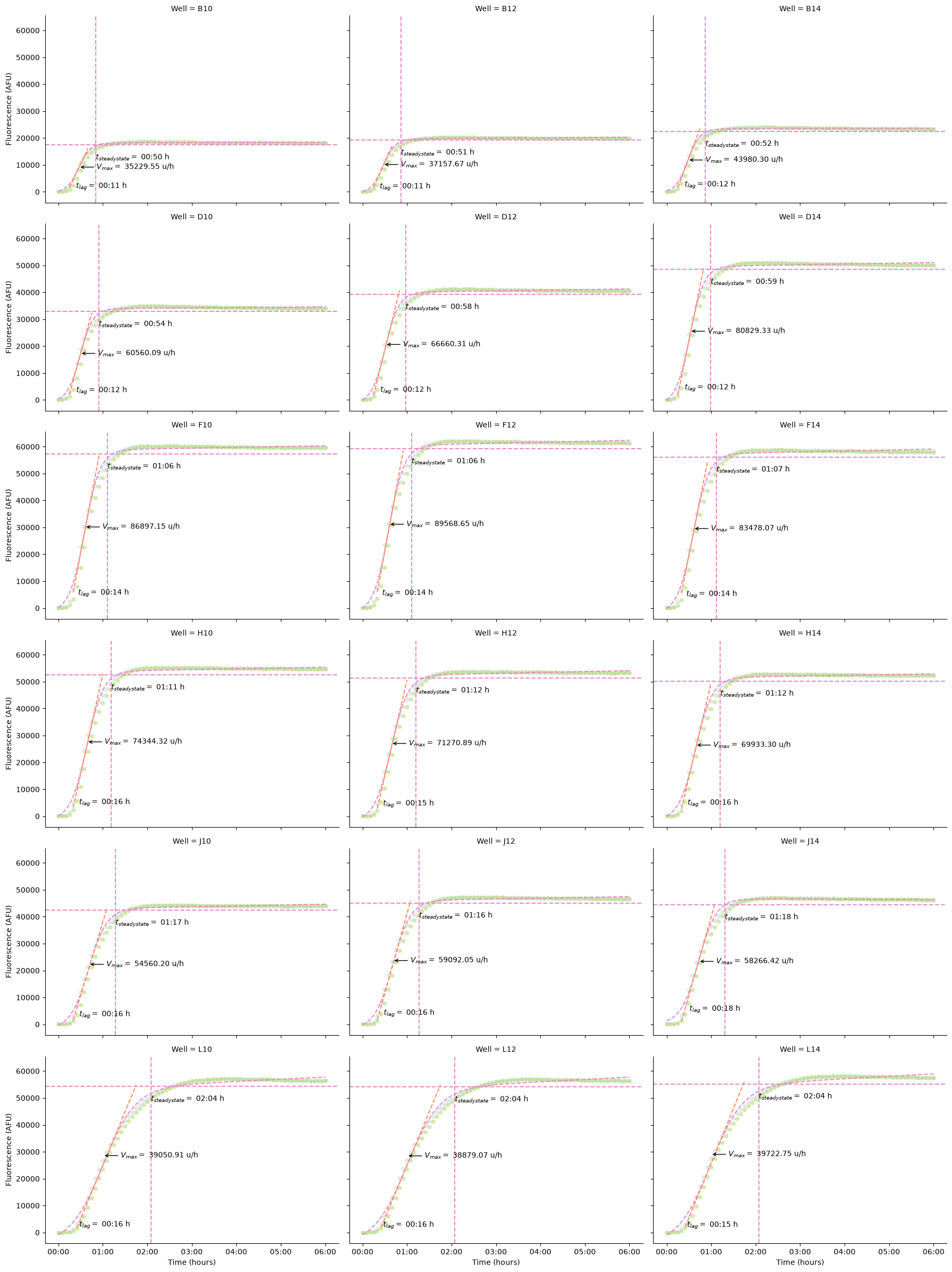
We can also calculate the kinetics and display the parameters as a table.
pr.kinetic_analysis(data)Loading...