!pip install nucleus-cdk==0.5.0rc2 | tail -n2

Requirement already satisfied: asttokens in /opt/homebrew/anaconda3/lib/python3.12/site-packages (from stack-data->ipython>=6.1.0->ipywidgets==8.*->jupyter-bokeh<5.0.0,>=4.0.5->nucleus-cdk==0.5.0rc2) (2.0.5)
Requirement already satisfied: pure-eval in /opt/homebrew/anaconda3/lib/python3.12/site-packages (from stack-data->ipython>=6.1.0->ipywidgets==8.*->jupyter-bokeh<5.0.0,>=4.0.5->nucleus-cdk==0.5.0rc2) (0.2.2)

%load_ext autoreload
%autoreload 2

from cdk.analysis.cytosol import platereader as pr
import warnings

# Ignore warnings
warnings.filterwarnings('ignore')

# Initialize plotting
pr.plot_setup()

Analysis: 20250811¶

All the data is in the same file, so I just updated the platemap to include everything and to add some extra labels we can slice the data by and to make the names simpler so that the legends are easier to interpret. The original spreadsheet is here on google drive.

platemap_path = "../Platemap (acjs)/20250811-acjs-PPK-platemap.tsv"
data_path = "../data/20250729-104410-cytation5-pure-timecourse-gfp--biotek-cdk.txt"

data, platemap = pr.load_platereader_data(data_path, platemap_path)

Plots¶

Make some timeseries plots. We can add extra parameters to slice the data different ways (like hue and col below). The plot_curves function takes the same parameters as relplot in Seaborn.

Make a plot per crowding molecule (col="Crowder"), coloring each line by the kind of metabolism (hue="Metabolism").

pr.plot_curves(data, hue="Metabolism", col="Crowder");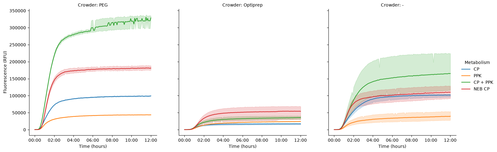

Swap them around, so we’re looking at the difference between crowders, split out by the kind of metabolism. It’s interesting that CP is really similar for both PEG and no crowder, while PEG solidly beats no crowder in the NEB positive.

pr.plot_curves(data, hue="Crowder", col="Metabolism");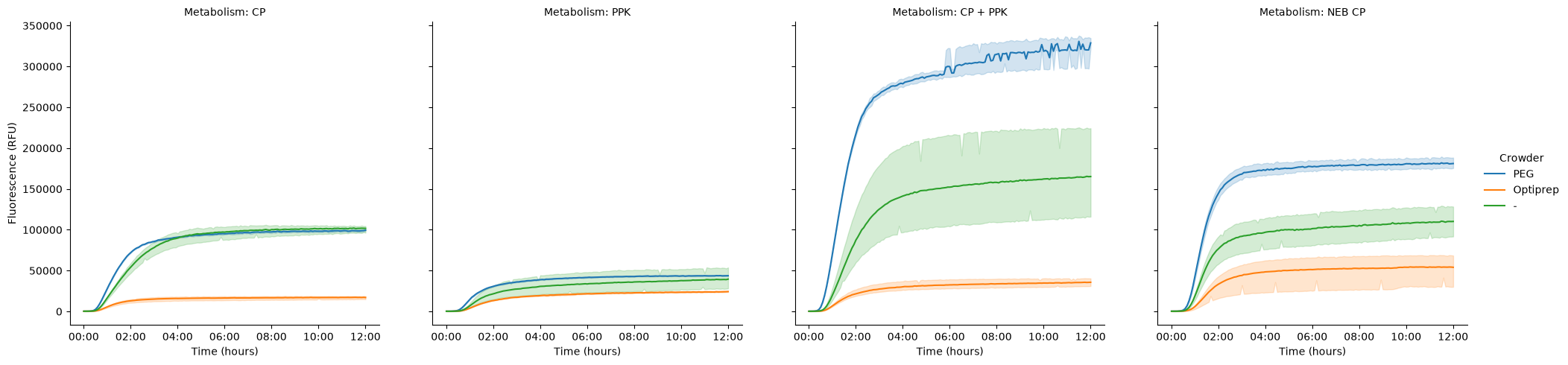

Replicates¶

Let’s take a look at the individual traces, to see where the wide errors on the traces are coming from.

pr.plot_curves(data, hue="Metabolism", col="Crowder", units="Well", estimator=None, facet_kws={"sharey":False});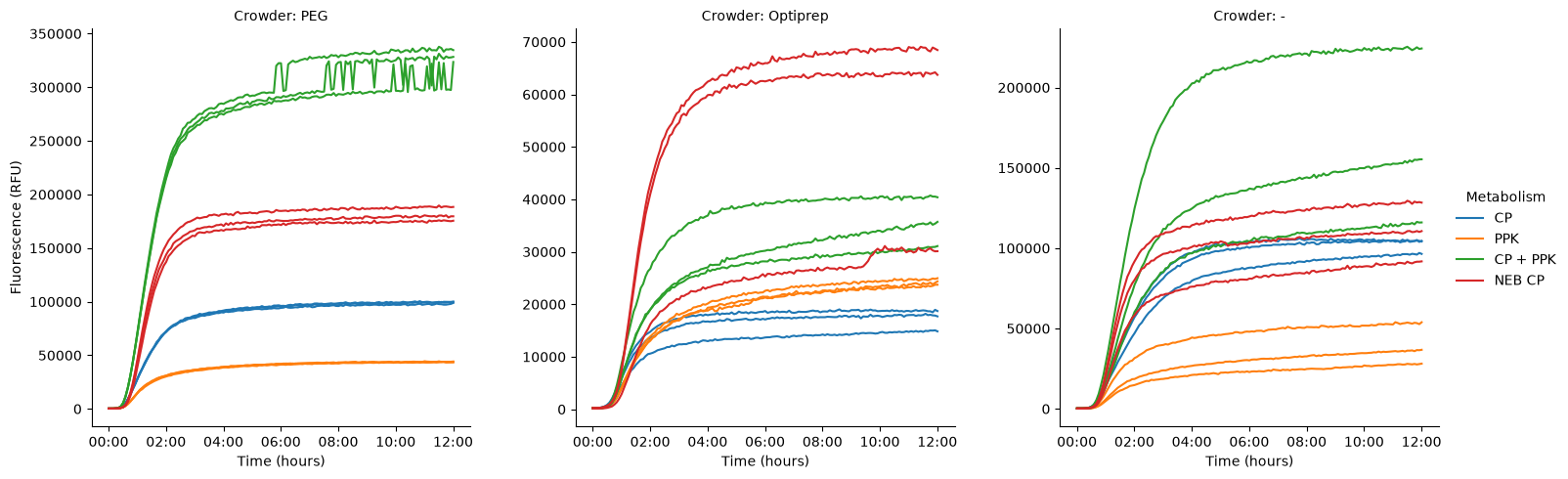

Looks like the variance is, in general, coming from either a very high or very low replicate within a set. In the Optiprep set, we see two nice high lines for the NEB positive, plus one weirdly low one. In the no-crowder set, we see a nice high curve for CP+PPK, and two lower curves, though they’re all kind of spread out. The three NEB positive lines are also spread out, though not so much.

The PEG lines are all nicely clustered, and we see the weird step change happen to all of them (at different times). Unclear what this is--worth digging into. Given the wells were in different parts of the plate, it’s also interesting to consider whether the higher variance is somehow coming from their location on plate.

Let’s plot them with a shared Y axis, just to see the variance, etc, in relation to the overall scale of the experiment as a whole.

pr.plot_curves(data, hue="Metabolism", col="Crowder", units="Well", estimator=None);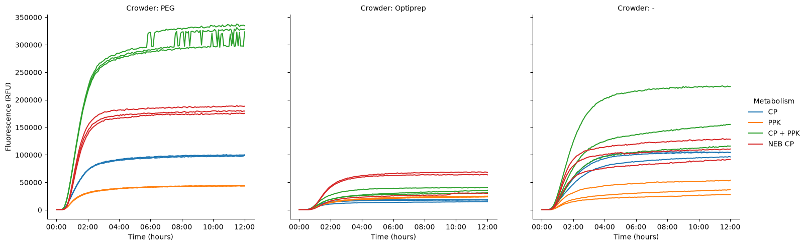

We can also crop back the time to ~steady state, so that we can better see differences in the early kinetic curve.

pr.plot_curves(data[data["Time"] < "5:00:00"], hue="Metabolism", col="Crowder", units="Well", estimator=None);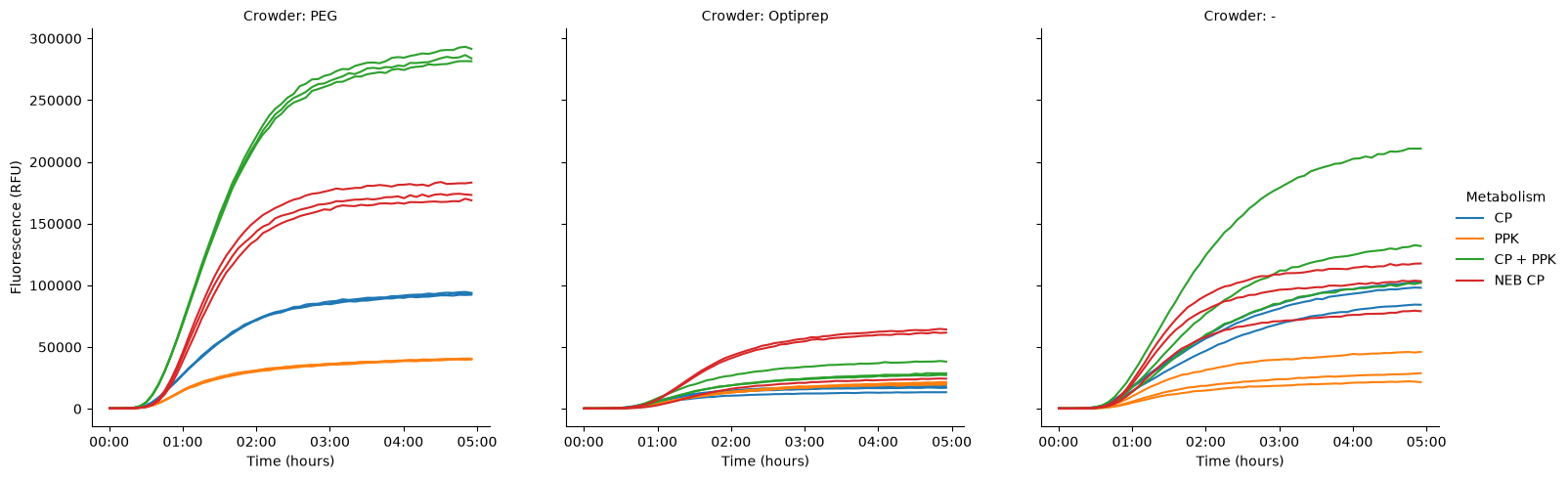

To really split it out, we could look at only the replicates for each Crowder-Metabolism pair, so we’re just looking at three lines per plot.

pr.plot_curves(data[data["Time"] < "5:00:00"], hue="Metabolism", row="Metabolism", col="Crowder", units="Well", estimator=None);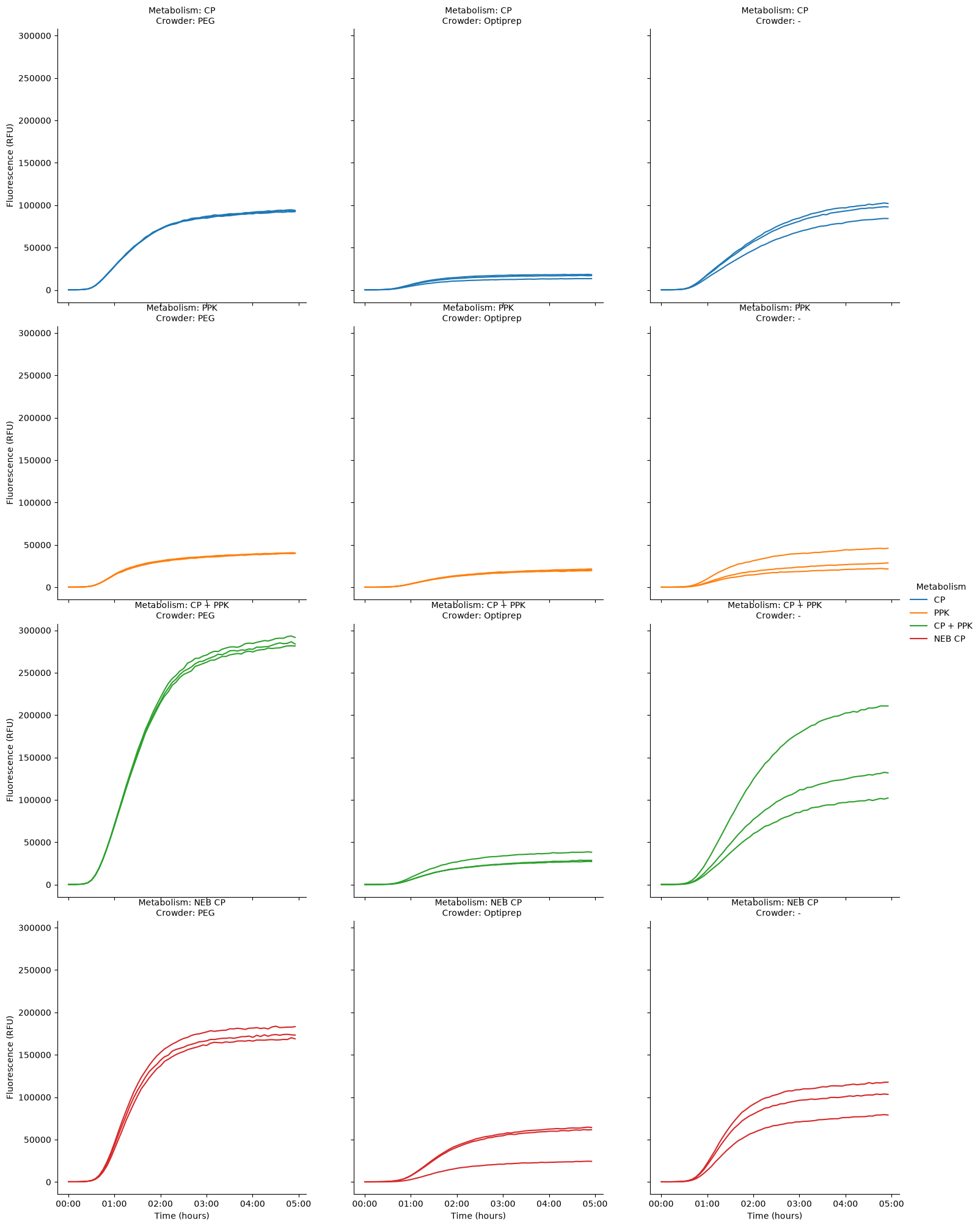

Steady state¶

Same as we did for the timeseries, this time doing the kind of metabolism on the x axis (x="Metabolism") and crowder as color (hue="Crowder").

# pr.plot_steadystate(data, x="Metabolism", hue="Crowder") - broken in installed nucleus-cdk: hue referencing a column other than x fails (the merge that restores full platemap columns was commented out upstream). Filed as https://github.com/bnext-bio/bnext/issues/67.

Swap them around like we did before, in case this is easier to read.

# pr.plot_steadystate(data, x="Crowder", hue="Metabolism") - broken in installed nucleus-cdk, see https://github.com/bnext-bio/bnext/issues/67

Make a plot like we had above, with one panel per crowder.

# pr.plot_steadystate(data, x="Metabolism", hue="Metabolism", col="Crowder", col_wrap=3) - broken in installed nucleus-cdk (col != x), see https://github.com/bnext-bio/bnext/issues/67

Error Bars¶

The error bars are noticeably smaller than what we’d guess by eye from the curves--why is this? By default, the error bars are plotting the 95% confidence interval--the range within which we expect the true mean falls. There are other ways to visualize the error. First, let’s look at what all the steady states look like (per well):

# pr.plot_steadystate(data, x="Well", hue="Metabolism", col="Crowder", col_wrap=3) - broken in installed nucleus-cdk (x="Well" duplicates the Well column internally), see https://github.com/bnext-bio/bnext/issues/67

This matches what we see in the curves more closely. The variance in some of the experiments looks a lot less bad, when scaled to the max of the best experiment (this might actually be kind of misleading though).

Let’s plot one of the earlier graphs, but with some different estimates of error/variance. Check out the seaborn documentation on uncertainty for an explanation of what these all are.

First, standard deviation:

# pr.plot_steadystate(data, x="Crowder", hue="Metabolism", errorbar="sd") - broken in installed nucleus-cdk, see https://github.com/bnext-bio/bnext/issues/67

This looks a lot more like we’re expecting. What about percent interval?

# pr.plot_steadystate(data, x="Crowder", hue="Metabolism", errorbar="pi") - broken in installed nucleus-cdk, see https://github.com/bnext-bio/bnext/issues/67

Also pretty solid. We can try the standard error:

# pr.plot_steadystate(data, x="Crowder", hue="Metabolism", errorbar="se") - broken in installed nucleus-cdk, see https://github.com/bnext-bio/bnext/issues/67

This is unsurprisingly similar to the 95% confidence interval, given our low number of samples. Overall, we should probably change the default errorbar estimator to the standard deviation, since it’s less surprising and we’re unlikely to have a large population in any sample (large number of replicates).

We can also provide a custom estimator--let’s use one that plots the range:

# pr.plot_steadystate(data, x="Crowder", hue="Metabolism", errorbar=lambda x: (x.min(), x.max())) - broken in installed nucleus-cdk, see https://github.com/bnext-bio/bnext/issues/67

Perhaps this is even better than the SD, since we know we’re likely to have 2-3, and probably at most 5, replicates of a given sample.

New feature inspired--let’s plot the raw data points (per well) on top of the bars:

# pr.plot_steadystate(data, x="Crowder", hue="Metabolism", show_points=True) - broken in installed nucleus-cdk, see https://github.com/bnext-bio/bnext/issues/67

Mg Concentration vs Optiprep¶

# pr.plot_steadystate(data, x="Crowder", hue="[Mg2+]", show_points=True) - broken in installed nucleus-cdk, see https://github.com/bnext-bio/bnext/issues/67

# pr.plot_steadystate(data, hue="[Mg2+]", col="Crowder", x="Type", sharey=False, show_points=True) - broken in installed nucleus-cdk, see https://github.com/bnext-bio/bnext/issues/67

Kinetics Analysis¶

Plot the overall kinetics. This plot is going to be huge, so we increase the number of columns we’re willing to make (col_wrap=4).

pr.plot_kinetics(data, col_wrap=3)

PROVIDING AVERAGED KINETICS

(<seaborn.axisgrid.FacetGrid at 0x15b25bc50>, Velocity \ Time Data Max Name Read CP GFP-Gext 0 days 01:56:49.703175980 51591.90 35360.10 CP (+Optiprep) GFP-Gext 0 days 01:09:25.838032851 8458.97 9526.62 CP (+PEG) GFP-Gext 0 days 01:20:01.629748317 50166.86 48561.41 CP + PPK GFP-Gext 0 days 02:08:00.636863372 82809.95 56270.27 CP + PPK (+Optiprep) GFP-Gext 0 days 01:39:44.298348783 17539.25 12935.71 CP + PPK (+PEG) GFP-Gext 0 days 01:35:50.167726917 157886.49 137146.38 NEB PURE GFP-Gext 0 days 01:36:21.250299620 52613.59 56607.93 NEB PURE (+Optiprep) GFP-Gext 0 days 01:35:28.257610413 25175.82 25756.01 NEB PURE (+PEG) GFP-Gext 0 days 01:21:08.673754170 90442.83 123669.83 PPK GFP-Gext 0 days 01:41:08.384407236 17557.66 12274.87 PPK (+Optiprep) GFP-Gext 0 days 01:23:20.693905149 10915.97 8093.92 PPK (+PEG) GFP-Gext 0 days 01:03:10.022932370 22526.63 20271.26 Lag \ Time Data Name Read CP GFP-Gext 0 days 00:27:19.894588486 8028.92 CP (+Optiprep) GFP-Gext 0 days 00:16:04.265767190 263.00 CP (+PEG) GFP-Gext 0 days 00:17:54.360516142 3439.90 CP + PPK GFP-Gext 0 days 00:35:45.635753486 19324.00 CP + PPK (+Optiprep) GFP-Gext 0 days 00:09:28.288103476 1192.66 CP + PPK (+PEG) GFP-Gext 0 days 00:25:28.324162910 28159.05 NEB PURE GFP-Gext 0 days 00:34:13.284258166 10375.23 NEB PURE (+Optiprep) GFP-Gext 0 days 00:38:58.318498164 2243.91 NEB PURE (+PEG) GFP-Gext 0 days 00:37:08.577876003 13799.56 PPK GFP-Gext 0 days 00:04:02.309376523 723.40 PPK (+Optiprep) GFP-Gext 0 days 00:02:27.233345294 -1128.51 PPK (+PEG) GFP-Gext -1 days +23:56:26.434985522 -3071.72 Steady State \ Time Data Name Read CP GFP-Gext 0 days 04:08:35.240033356 98024.62 CP (+Optiprep) GFP-Gext 0 days 02:27:59.255118903 16072.05 CP (+PEG) GFP-Gext 0 days 02:51:28.988154378 95317.04 CP + PPK GFP-Gext 0 days 04:23:49.373371663 157338.90 CP + PPK (+Optiprep) GFP-Gext 0 days 03:52:37.854187041 33324.58 CP + PPK (+PEG) GFP-Gext 0 days 03:19:25.648102959 299984.33 NEB PURE GFP-Gext 0 days 03:07:49.634561931 99965.82 NEB PURE (+Optiprep) GFP-Gext 0 days 02:58:38.992038866 47834.05 NEB PURE (+PEG) GFP-Gext 0 days 02:25:55.474359636 171841.38 PPK GFP-Gext 0 days 04:04:05.645614387 33359.56 PPK (+Optiprep) GFP-Gext 0 days 03:22:26.053132090 20740.34 PPK (+PEG) GFP-Gext 0 days 02:41:24.183135436 42800.59 Fit \ params Name Read CP GFP-Gext [103183.80800694443, 1.3638951482093218, 1.947... CP (+Optiprep) GFP-Gext [16917.947542481445, 2.2519109768946213, 1.157... CP (+PEG) GFP-Gext [100333.7237300093, 1.9358327412397578, 1.3337... CP + PPK GFP-Gext [165619.89416766114, 1.3220869666802362, 2.133... CP + PPK (+Optiprep) GFP-Gext [35078.50524063764, 1.4809557407865335, 1.6623... CP + PPK (+PEG) GFP-Gext [315772.98297645064, 1.7530837886695363, 1.597... NEB PURE GFP-Gext [105227.17453979472, 2.1023012948577042, 1.605... NEB PURE (+Optiprep) GFP-Gext [50351.63281804238, 2.1507410688575415, 1.5911... NEB PURE (+PEG) GFP-Gext [180885.66372570998, 2.732172159936075, 1.3524... PPK GFP-Gext [35115.324006220464, 1.4523784230071486, 1.685... PPK (+Optiprep) GFP-Gext [21831.942094714865, 1.4884168588966713, 1.389... PPK (+PEG) GFP-Gext [45053.25425913357, 1.7995590841605449, 1.0527... R^2 drift Name Read CP GFP-Gext 0.99 139.58 CP (+Optiprep) GFP-Gext 1.00 196.79 CP (+PEG) GFP-Gext 0.99 623.64 CP + PPK GFP-Gext 0.97 -726.40 CP + PPK (+Optiprep) GFP-Gext 0.98 252.75 CP + PPK (+PEG) GFP-Gext 0.96 549.15 NEB PURE GFP-Gext 0.97 326.59 NEB PURE (+Optiprep) GFP-Gext 1.00 777.44 NEB PURE (+PEG) GFP-Gext 0.99 717.21 PPK GFP-Gext 0.98 608.31 PPK (+Optiprep) GFP-Gext 1.00 551.65 PPK (+PEG) GFP-Gext 0.99 699.67 )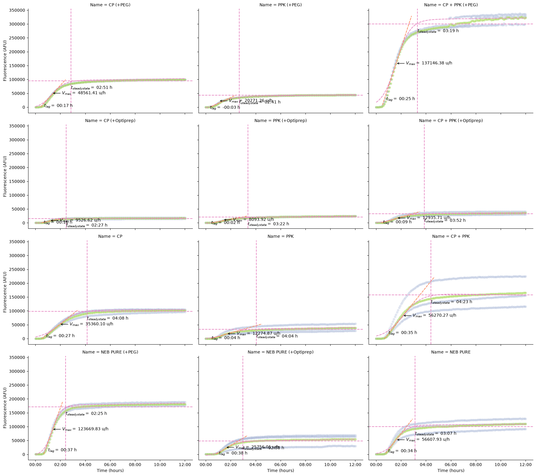

pr.plot_kinetics(data, col_wrap=3, sharey=False)

PROVIDING AVERAGED KINETICS

(<seaborn.axisgrid.FacetGrid at 0x159571310>, Velocity \ Time Data Max Name Read CP GFP-Gext 0 days 01:56:49.703175980 51591.90 35360.10 CP (+Optiprep) GFP-Gext 0 days 01:09:25.838032851 8458.97 9526.62 CP (+PEG) GFP-Gext 0 days 01:20:01.629748317 50166.86 48561.41 CP + PPK GFP-Gext 0 days 02:08:00.636863372 82809.95 56270.27 CP + PPK (+Optiprep) GFP-Gext 0 days 01:39:44.298348783 17539.25 12935.71 CP + PPK (+PEG) GFP-Gext 0 days 01:35:50.167726917 157886.49 137146.38 NEB PURE GFP-Gext 0 days 01:36:21.250299620 52613.59 56607.93 NEB PURE (+Optiprep) GFP-Gext 0 days 01:35:28.257610413 25175.82 25756.01 NEB PURE (+PEG) GFP-Gext 0 days 01:21:08.673754170 90442.83 123669.83 PPK GFP-Gext 0 days 01:41:08.384407236 17557.66 12274.87 PPK (+Optiprep) GFP-Gext 0 days 01:23:20.693905149 10915.97 8093.92 PPK (+PEG) GFP-Gext 0 days 01:03:10.022932370 22526.63 20271.26 Lag \ Time Data Name Read CP GFP-Gext 0 days 00:27:19.894588486 8028.92 CP (+Optiprep) GFP-Gext 0 days 00:16:04.265767190 263.00 CP (+PEG) GFP-Gext 0 days 00:17:54.360516142 3439.90 CP + PPK GFP-Gext 0 days 00:35:45.635753486 19324.00 CP + PPK (+Optiprep) GFP-Gext 0 days 00:09:28.288103476 1192.66 CP + PPK (+PEG) GFP-Gext 0 days 00:25:28.324162910 28159.05 NEB PURE GFP-Gext 0 days 00:34:13.284258166 10375.23 NEB PURE (+Optiprep) GFP-Gext 0 days 00:38:58.318498164 2243.91 NEB PURE (+PEG) GFP-Gext 0 days 00:37:08.577876003 13799.56 PPK GFP-Gext 0 days 00:04:02.309376523 723.40 PPK (+Optiprep) GFP-Gext 0 days 00:02:27.233345294 -1128.51 PPK (+PEG) GFP-Gext -1 days +23:56:26.434985522 -3071.72 Steady State \ Time Data Name Read CP GFP-Gext 0 days 04:08:35.240033356 98024.62 CP (+Optiprep) GFP-Gext 0 days 02:27:59.255118903 16072.05 CP (+PEG) GFP-Gext 0 days 02:51:28.988154378 95317.04 CP + PPK GFP-Gext 0 days 04:23:49.373371663 157338.90 CP + PPK (+Optiprep) GFP-Gext 0 days 03:52:37.854187041 33324.58 CP + PPK (+PEG) GFP-Gext 0 days 03:19:25.648102959 299984.33 NEB PURE GFP-Gext 0 days 03:07:49.634561931 99965.82 NEB PURE (+Optiprep) GFP-Gext 0 days 02:58:38.992038866 47834.05 NEB PURE (+PEG) GFP-Gext 0 days 02:25:55.474359636 171841.38 PPK GFP-Gext 0 days 04:04:05.645614387 33359.56 PPK (+Optiprep) GFP-Gext 0 days 03:22:26.053132090 20740.34 PPK (+PEG) GFP-Gext 0 days 02:41:24.183135436 42800.59 Fit \ params Name Read CP GFP-Gext [103183.80800694443, 1.3638951482093218, 1.947... CP (+Optiprep) GFP-Gext [16917.947542481445, 2.2519109768946213, 1.157... CP (+PEG) GFP-Gext [100333.7237300093, 1.9358327412397578, 1.3337... CP + PPK GFP-Gext [165619.89416766114, 1.3220869666802362, 2.133... CP + PPK (+Optiprep) GFP-Gext [35078.50524063764, 1.4809557407865335, 1.6623... CP + PPK (+PEG) GFP-Gext [315772.98297645064, 1.7530837886695363, 1.597... NEB PURE GFP-Gext [105227.17453979472, 2.1023012948577042, 1.605... NEB PURE (+Optiprep) GFP-Gext [50351.63281804238, 2.1507410688575415, 1.5911... NEB PURE (+PEG) GFP-Gext [180885.66372570998, 2.732172159936075, 1.3524... PPK GFP-Gext [35115.324006220464, 1.4523784230071486, 1.685... PPK (+Optiprep) GFP-Gext [21831.942094714865, 1.4884168588966713, 1.389... PPK (+PEG) GFP-Gext [45053.25425913357, 1.7995590841605449, 1.0527... R^2 drift Name Read CP GFP-Gext 0.99 139.58 CP (+Optiprep) GFP-Gext 1.00 196.79 CP (+PEG) GFP-Gext 0.99 623.64 CP + PPK GFP-Gext 0.97 -726.40 CP + PPK (+Optiprep) GFP-Gext 0.98 252.75 CP + PPK (+PEG) GFP-Gext 0.96 549.15 NEB PURE GFP-Gext 0.97 326.59 NEB PURE (+Optiprep) GFP-Gext 1.00 777.44 NEB PURE (+PEG) GFP-Gext 0.99 717.21 PPK GFP-Gext 0.98 608.31 PPK (+Optiprep) GFP-Gext 1.00 551.65 PPK (+PEG) GFP-Gext 0.99 699.67 )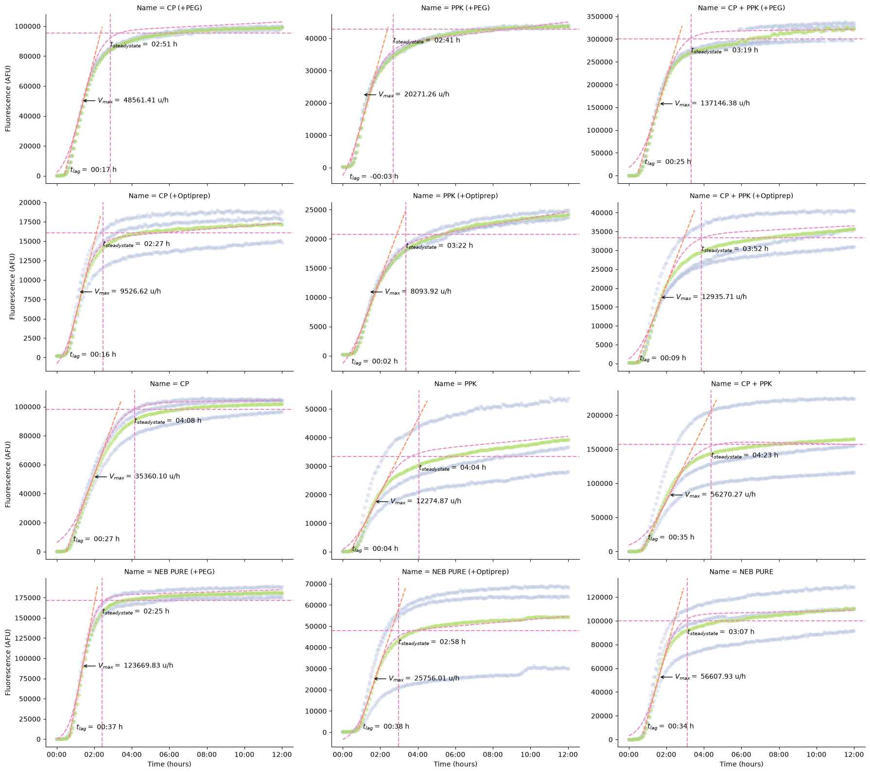

We don’t have specific functions yet, but we can also use the kinetic analysis table to drill into some specifics (like how long each well takes to get to steady state).

import seaborn as sns

data["Velocity"] = data["Data"].diff()
g = sns.relplot(
    data=data[(data["Time"] > "00:00:30") & (data["Time"] <= "5:00:00")], 
    x="Time", 
    y="Velocity", 
    hue="Metabolism", 
    col="Crowder", 
    kind="line")
pr._plot_timedelta(g)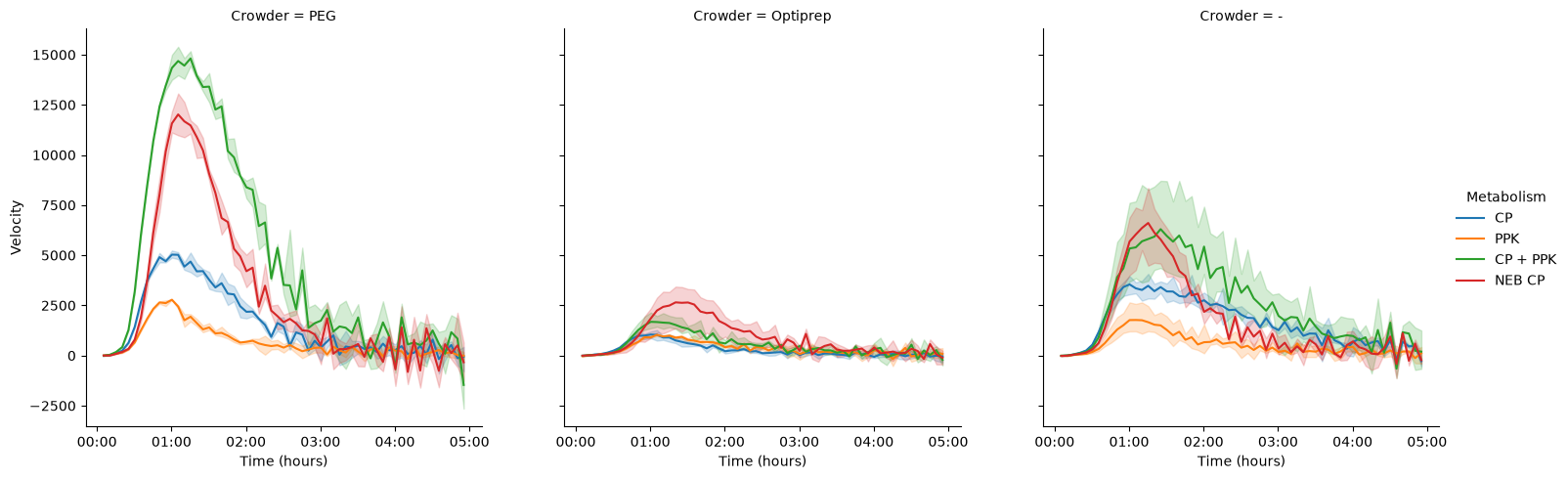

kinetics = pr.kinetic_analysis(data)
kinetics

import pandas as pd
import matplotlib.pyplot as plt
import seaborn as sns

g = sns.catplot(data=kinetics["Steady State"], y="Time", x="Name", kind="bar", orient="v", aspect=2)

# The names are still kind of long, so we need to rotate them in order to read them properly.
g.set_xticklabels(rotation=90)

<seaborn.axisgrid.FacetGrid at 0x15fd347d0>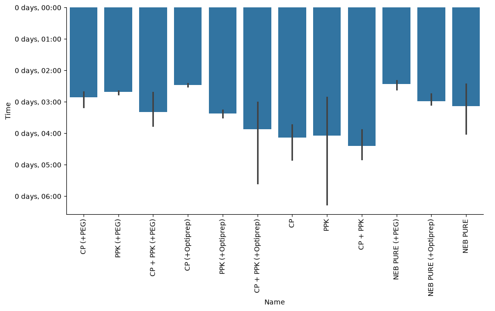

Quick experiment to see if there is some spatial effect to the variance on the plate. It doesn’t particularly look like it, though I could belive that it’s getting kind of worse as we go down from row B, to C, to D.

ss = pr.find_steady_state(data, group_by=["Well"]).reset_index()
ss["Row"] = ss["Well"].str[:1]
ss["Col"] = pd.to_numeric(ss["Well"].str[1:])
sns.heatmap(ss.pivot(index="Row", columns="Col", values="Data_steadystate"))

<Axes: xlabel='Col', ylabel='Row'>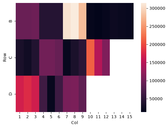

Summary¶

Overall summary of experiment

pr.plot_summary(data)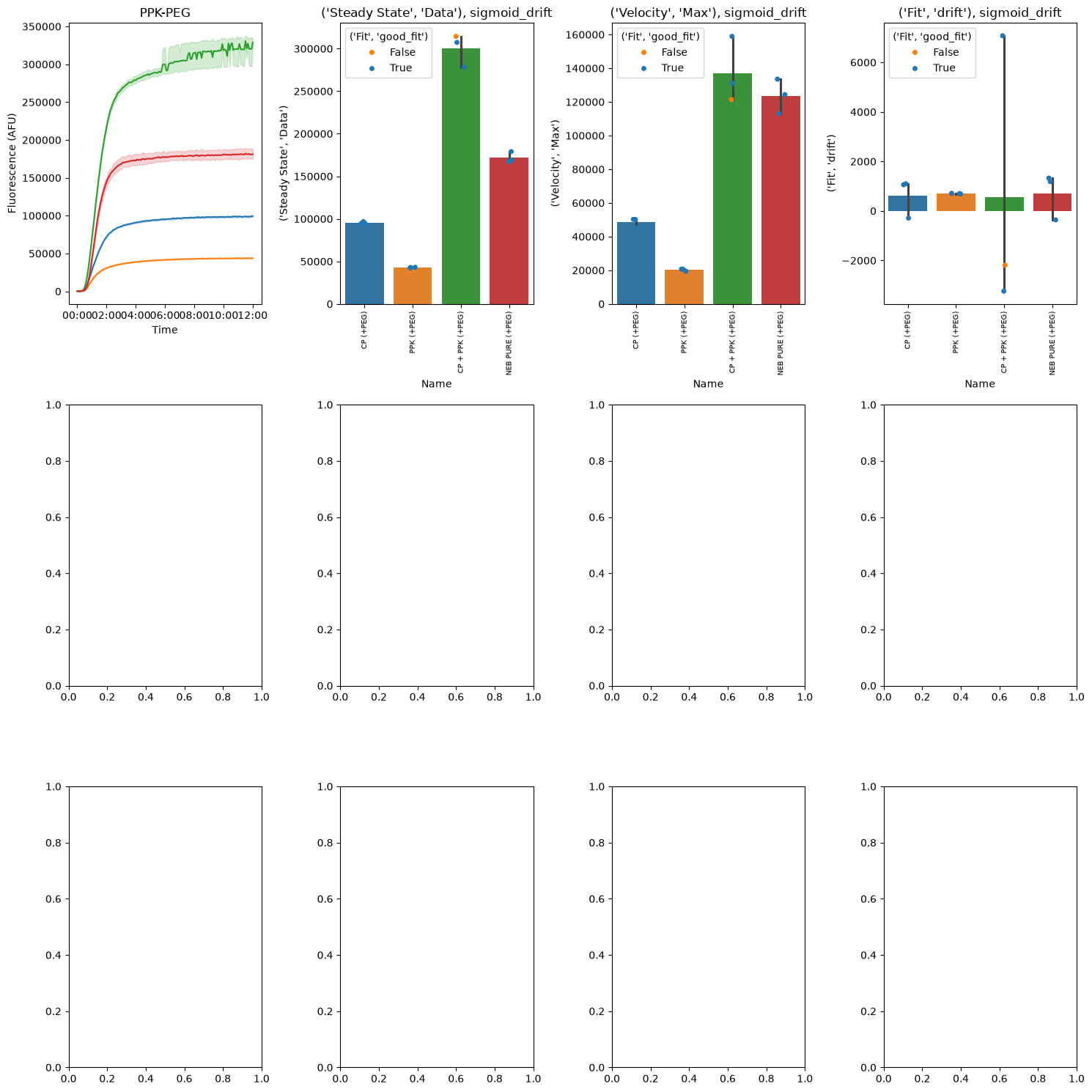

<Figure size 640x480 with 0 Axes>

<Figure size 640x480 with 0 Axes>

df = data[data["Experiment"] == "PPK"]
kinetics = pr.kinetic_analysis(df, ["Name"])
kinetics
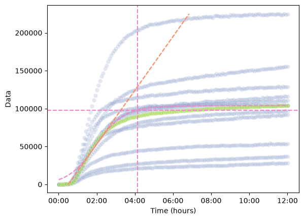
pr.plot_kinetics_by_well(
    data=df,
    kinetics=kinetics,
    group_by=["Name"],
    show_mean=True,
    show_fit=True,
    annotate=False,
    hue="Name"
)

PROVIDING AVERAGED KINETICS

import matplotlib.pyplot as plt
import pandas as pd

fig, ax = plt.subplots()
ax.axis('off')
pd.plotting.table(ax, pr.kinetic_analysis(df))