

AmajLime analysis
!pip install nucleus-cdk==0.5.0rc2 | tail -n2Requirement already satisfied: asttokens in /opt/homebrew/anaconda3/lib/python3.12/site-packages (from stack-data->ipython>=6.1.0->ipywidgets==8.*->jupyter-bokeh<5.0.0,>=4.0.5->nucleus-cdk==0.5.0rc2) (2.0.5)
Requirement already satisfied: pure-eval in /opt/homebrew/anaconda3/lib/python3.12/site-packages (from stack-data->ipython>=6.1.0->ipywidgets==8.*->jupyter-bokeh<5.0.0,>=4.0.5->nucleus-cdk==0.5.0rc2) (0.2.2)
Dataframe construction
The data analysed in this notebook was generated from an endpoint fluorescent measurement. The data was parsed from the original .txt file to create the following dataframe.
import pandas as pd
import matplotlib.pyplot as plt
import seaborn as sns

import warnings
warnings.filterwarnings('ignore', category=FutureWarning)

data_structure = {
 'Number': [1, 1, 1, 2, 2, 2, 3, 3, 3, 4, 4, 4, 5, 5, 5, 6, 6, 6, 7, 7, 7, 8, 8, 8, 9, 9, 9, 10, 10, 10, 11, 11, 11],
 'Sample': ['Negative', 'Negative', 'Negative', 'T7-1', 'T7-1', 'T7-1', 'T7-2', 'T7-2', 'T7-2', 'T7-3', 'T7-3', 'T7-3', 'T7-4', 'T7-4', 'T7-4', 'T7-5', 'T7-5', 'T7-5', 'T7-6', 'T7-6', 'T7-6', 'T7-7', 'T7-7', 'T7-7', 'T7-8', 'T7-8', 'T7-8', 'T7-9', 'T7-9', 'T7-9', 'T7-10', 'T7-10', 'T7-10'],
 'Fluorescence Units': [6070.0, 6233.0, 6261.0, 4380.0, 6351.0, 2616.0, 6449.0, 6562.0, 6224.0, 19444.0, 20506.0, 18755.0, 7198.0, 6906.0, 6796.0, 45736.0, 43061.0, 47363.0, 27326.0, 31660.0, 30357.0, 13390.0, 12505.0, 11574.0, 442462.0, 442018.0, 427332.0, 1098370.0, 1047753.0, 1026269.0, 1026679.0, 992618.0, 1026745.0]
}


data = pd.DataFrame(data_structure)

#data.head
Background subtraction
A new column was added to the dataframe,“blanked”, in which the mean fluorescence value of the “Negative” replicates was substracted from the fluorescence values of all samples.
background = data.loc[data["Sample"] == "Negative", "Fluorescence Units"].mean()

data["Blanked"] = data["Fluorescence Units"] - background

data.head
<bound method NDFrame.head of Number Sample Fluorescence Units Blanked
0 1 Negative 6070.0 -118.0
1 1 Negative 6233.0 45.0
2 1 Negative 6261.0 73.0
3 2 T7-1 4380.0 -1808.0
4 2 T7-1 6351.0 163.0
5 2 T7-1 2616.0 -3572.0
6 3 T7-2 6449.0 261.0
7 3 T7-2 6562.0 374.0
8 3 T7-2 6224.0 36.0
9 4 T7-3 19444.0 13256.0
10 4 T7-3 20506.0 14318.0
11 4 T7-3 18755.0 12567.0
12 5 T7-4 7198.0 1010.0
13 5 T7-4 6906.0 718.0
14 5 T7-4 6796.0 608.0
15 6 T7-5 45736.0 39548.0
16 6 T7-5 43061.0 36873.0
17 6 T7-5 47363.0 41175.0
18 7 T7-6 27326.0 21138.0
19 7 T7-6 31660.0 25472.0
20 7 T7-6 30357.0 24169.0
21 8 T7-7 13390.0 7202.0
22 8 T7-7 12505.0 6317.0
23 8 T7-7 11574.0 5386.0
24 9 T7-8 442462.0 436274.0
25 9 T7-8 442018.0 435830.0
26 9 T7-8 427332.0 421144.0
27 10 T7-9 1098370.0 1092182.0
28 10 T7-9 1047753.0 1041565.0
29 10 T7-9 1026269.0 1020081.0
30 11 T7-10 1026679.0 1020491.0
31 11 T7-10 992618.0 986430.0
32 11 T7-10 1026745.0 1020557.0>Plotting: AmajLime summary plot
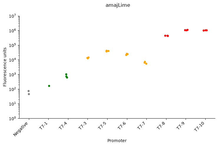
The plot order and color map is first defined to categorise the reporters into color coded low, medium, and high expression level groups. This enables easier visualisation of the dataset. The endpoint background substracted fluorescence units are then plotted for each promoter. A scatter plot is used to illustrate the overall spread of the data.
plot_order = [
    'Negative',
    'T7-1',
    'T7-4',
    'T7-3',
    'T7-5',
    'T7-6',
    'T7-7',
   'T7-8',
   'T7-9',
    'T7-10'
]

color_map = {
    'Negative': 'grey',
    'T7-1': 'green',
    'T7-4': 'green',
    'T7-3': 'orange',
    'T7-5': 'orange',
    'T7-6': 'orange',
    'T7-7': 'orange',
    'T7-8': 'red',
    'T7-9': 'red',
    'T7-10': 'red'
}

amajLime_plot=sns.catplot(
    data=data,
    x='Sample',
    y='Blanked',
    order=plot_order,
    palette=color_map,
    kind='strip',
    height=5,
    aspect=1.5
)

amajLime_plot.fig.suptitle('amajLime', x=0.54)
amajLime_plot.set_axis_labels('Promoter', 'Fluorescence units')
amajLime_plot.set_xticklabels(rotation=45, ha='right')
amajLime_plot.set(yscale="log", ylim=(1, 10000000))

plt.tight_layout()
amajLime_plot.savefig('Summary_data_amajLime.png', dpi=600)