Intro to Kinetics Analysis of Plate Reader Experiments

Sharon Newman

Kinetics Analysis Tutorial

This tutorial guides you through analyzing timeseries fluorescence data from in vitro protein expression experiments. We’ll cover data loading, normalization, visualization, kinetic parameter fitting, and summary statistics.

Table of Contents¶

1. Setup¶

First, import the necessary libraries and set up the plotting environment.

The custom platereader module that contains specialized functions for loading plate reader data, performing kinetic analysis, and visualization. The plot_setup() function configures matplotlib for time-series plots.

!pip install nucleus-cdk==0.5.0rc2 | tail -n2

# Surface a failed install here, rather than as a confusing ModuleNotFoundError
# in the import cell below.
import importlib.metadata as md
assert md.version("nucleus-cdk") == "0.5.0rc2", f"got {md.version('nucleus-cdk')}"

Requirement already satisfied: asttokens in /opt/homebrew/anaconda3/lib/python3.12/site-packages (from stack-data->ipython>=6.1.0->ipywidgets==8.*->jupyter-bokeh<5.0.0,>=4.0.5->nucleus-cdk==0.5.0rc2) (2.0.5)
Requirement already satisfied: pure-eval in /opt/homebrew/anaconda3/lib/python3.12/site-packages (from stack-data->ipython>=6.1.0->ipywidgets==8.*->jupyter-bokeh<5.0.0,>=4.0.5->nucleus-cdk==0.5.0rc2) (0.2.2)

%load_ext autoreload
%autoreload 2
    
import pandas as pd
import seaborn as sns
import matplotlib.pyplot as plt

# Import the cdk platereader module
from cdk.analysis.cytosol import platereader as pr

# Set up plotting
pr.plot_setup()

2. Load Data¶

Load your plate reader data and merge it with the platemap that describes experimental conditions.

data_file is the location of your platereader data (ideally in biotek-cdk format)
platemap_file: location of your platemap CSV with Well and experimental conditions
load_platereader_data() reads your plate reader output file and parses it into a standardized format with the platemap integrated
The resulting DataFrame contains columns: Date, Experiment, Plate, Well, Row, Column, Time, Read, Data, plus any columns from your platemap
Data column contains fluorescence measurements
Time representing elapsed time

# Specify file paths
data_file = "cytation5-pure-timecourse-gfp-biotek-cdk.txt"
platemap_file = "platemap.csv"


# Load data
data, platemap = pr.load_platereader_data(
    data_file=data_file,
    platemap_file=platemap_file,
    platereader="biotek-cdk"  # Options: "cytation", "envision", "biotek-cdk"
)

data.info()

<class 'pandas.core.frame.DataFrame'>
RangeIndex: 576 entries, 0 to 575
Data columns (total 30 columns):
 #   Column                       Non-Null Count  Dtype          
---  ------                       --------------  -----          
 0   Time                         576 non-null    timedelta64[ns]
 1   Well                         576 non-null    object         
 2   Data                         576 non-null    float64        
 3   Row                          576 non-null    object         
 4   Column                       576 non-null    int64          
 5   Read                         576 non-null    object         
 6   Plate                        576 non-null    object         
 7   Clock Time                   576 non-null    datetime64[ns] 
 8   Date                         576 non-null    object         
 9   Experiment                   576 non-null    object         
 10  Name                         576 non-null    object         
 11  Type                         576 non-null    object         
 12  PMix ID                      0 non-null      float64        
 13  [PMix] (mg/mL)               0 non-null      float64        
 14  Ribosome ID                  0 non-null      float64        
 15  [Ribosome] (uM)              0 non-null      float64        
 16  SMS ID                       0 non-null      float64        
 17  tRNA ID                      0 non-null      float64        
 18  [tRNA] (ug/uL)               0 non-null      float64        
 19  DNA ID                       0 non-null      float64        
 20  [DNA] (ng/uL)                0 non-null      float64        
 21  PMix Vol (uL)                0 non-null      float64        
 22  Ribosome Vol (uL)            0 non-null      float64        
 23  SMS Vol (uL)                 0 non-null      float64        
 24  tRNA Vol (uL)                0 non-null      float64        
 25  DNA Vol (uL)                 0 non-null      float64        
 26  RNase Inhib Vol (uL)         0 non-null      float64        
 27  Water vol (uL)               0 non-null      float64        
 28  Rxn Volume (uL)              576 non-null    int64          
 29  Standard Concentration [nM]  384 non-null    float64        
dtypes: datetime64[ns](1), float64(18), int64(2), object(8), timedelta64[ns](1)
memory usage: 135.1+ KB

3. Plot Raw Curves¶

Visualize the time-series fluorescence data to inspect curve shapes and identify any issues.

plot_curves_by_name() creates line plots with time on x-axis and fluorescence (Data) on y-axis
Each line represents one well, colored by the Name column (experimental condition)
If you have multiple gain data, they’ll be plotted in separate subplots (but you should choose one to move forward with)
This visualization helps you spot outliers, failed reactions, or unexpected kinetics before fitting

g = pr.plot_curves(data=data, y="Data")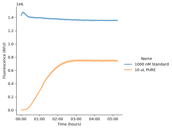

4. Normalize Data¶

Normalize your data to an internal fluorescence sample so that you have relative fluorescence to compare to other experiments.

data = pr.normalize_data_to_controls(data, ctrl_name = '1000 nM Standard')

Data Normalized to 1000 nM Standard in col data_normalized. The active column for subsequent operations is: data_normalized

Now replot your curves to see them normalized

g = pr.plot_curves(data=data)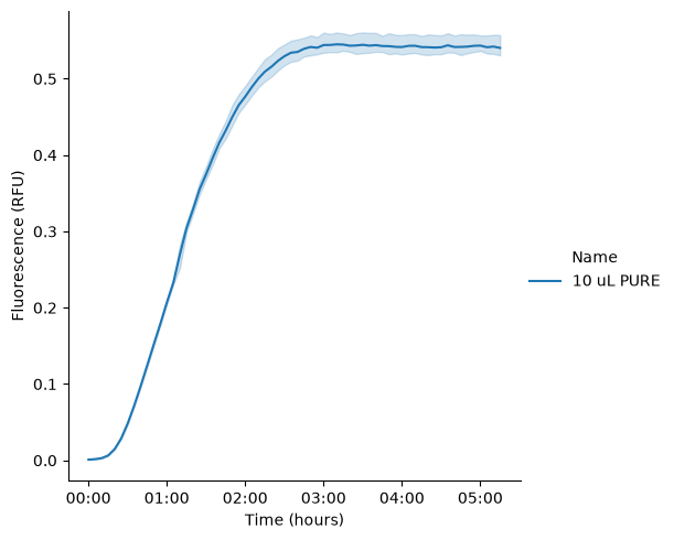

5. Kinetic Analysis¶

Fit sigmoid curves to the data to extract kinetic parameters: maximum reaction rate ( $V_\text{max}$ ), lag time, steady-state fluorescence, and drift.

kinetic_analysis() fits a logistic curve (with optional drift term) to each replicate well.

F(t) = F_\text{ss}\frac{1}{1 + e^{-k(t-\tau_\text{vel})}} + d(t- \tau_\text{drift}),

(1)

with the following parameters:

Fit Parameter	Name	Units	What it tells you
$F_\text{ss}$	Steady-State Fluorescence	$u$	Fluorescence at completion of the reaction. Proportional to total amount of reporter expressed.
$k$	Steepness	unitless	How fast is the reaction?
$\tau_\text{vel}$	Inflection Time	$h$	How long until the reaction reaches its fastest rate?
$d$	Drift Rate	$u \cdot h^{-1}$	The rate of drift after steady state (ideally, close to zero).
$\tau_\text{drift}$	Drift Onset Time	$h$	When does drift start to affect fluorescence?

Metrics extracted:

Maximum reaction rate ( $V_\text{max}$ ): the maximum slope of the sigmoid, which occurs at $\tau_\text{vel}$ and equals $\frac{F_\text{ss} \cdot k}{4}$ . This is not the Michaelis–Menten $V_\text{max}$ . Use $\frac{F_\text{ss} \cdot k}{4}$ for downstream calculations that require a slope with units ( $u \cdot h^{-1}$ ). When comparing reaction rates across conditions, use $k$ instead.
Lag time ( $\tau_\text{lag}$ ): the time it takes for the reaction to “start” (units of $h$ ). Explicitly, the x-intercept of the line tangent to the inflection point ( $\tau_{vel}$ ) on the sigmoid. This is metric is related to transcription lag time, translation lag time, and the maturation time of your reporter.
Time-to-completion ( $\tau_\text{ss}$ ): the time at which the reaction is “finished” (units of $h$ ). Explicitly, when the sigmoid reaches a chosen fraction $\alpha$ of its asymptote (default $\alpha=0.95$ ). $\tau_\text{ss}$ can be derived analytically from the model as
$\tau_\text{ss} \;=\; t_0 + \frac{1}{k}\ln\!\left(\frac{\alpha}{1-\alpha}\right).$
(2)
R²: Goodness of fit

# Perform kinetic analysis using sigmoid_drift model
kinetics = pr.kinetic_analysis(
    data=data,
    group_by=['Name'],  # Group by experimental condition
)

kinetics

PROVIDING AVERAGED KINETICS

Loading...

Visualize Fits on Individual Wells¶

What’s happening:

plot_kinetics_by_well() overlays fitted curves and kinetic parameters on raw data
Visual inspection ensures fits are reasonable (high R², smooth curves)
Annotations show where Vmax, lag time, and steady-state occur

# Plot kinetic fits
sample = data[data["Type"] == "Sample"]
g, kinetics = pr.plot_kinetics(sample, kinetics=kinetics, group_by=["Name"])
plt.savefig("../assets/thumbnail.png")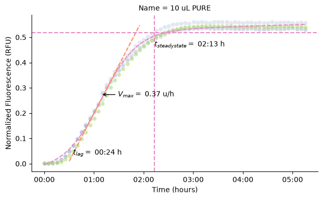

6. Summary Plots¶

Compare kinetic parameters across experimental conditions. The plot_kinetics_summary() function creates a comprehensive multi-panel figure with raw curves, steady-state fluorescence, $V_\text{max}$ , and drift rate. Error bars show std across technical replicates

pr.plot_summary(data)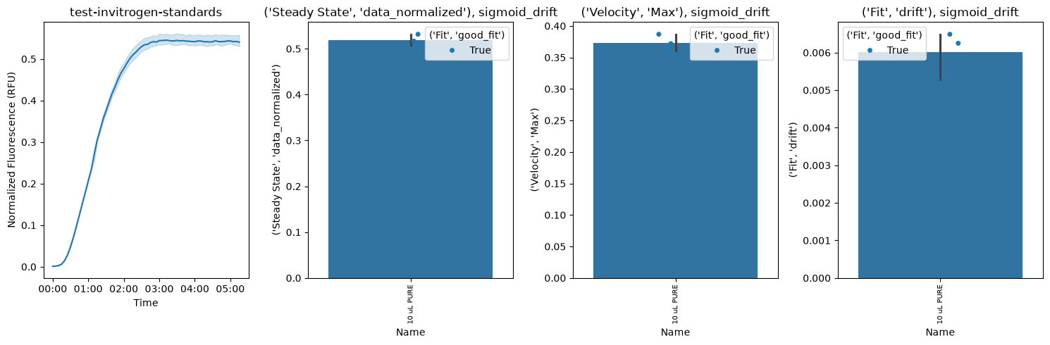

Key Metrics Explained¶

1. Steady-State Fluorescence¶

The fluorescence value reached at the completion of the reaction, with units: fluorescence units (e.g., a.u., RFU, $\mu$ M GFP, etc.).
Proxy for the total amount of protein produced. Higher values indicate greater expression yield.
Estimated as the asymptotic behavior of the logistic curve (ignoring drift).

2. Maximum Velocity¶

The steepest slope of the fluorescence curve (at the inflection point), with units: fluorescence units per time.
Reflects the peak rate of protein synthesis.
Sensitive to enzyme activity, substrate availability, and reaction conditions.

3. Lag Time¶

Time before exponential fluorescence increase begins, with units: time.
May reflect time for initial reaction steps (e.g., transcription, ribosome assembly, etc.).
Shorter lag times suggest faster reaction initiation.

4. Drift¶

Rate of fluorescence change after reaching steady-state, with units: fluorescence units per time.
Positive drift: continued synthesis or aggregation, evaporation.
Negative drift: photobleaching, protein degradation, or quenching

5. R² Value¶

Goodness of fit (0 to 1, higher is better), with units: unitless.
R² > 0.98 indicates excellent fit
Poor fits may indicate noisy data, overflow errors, or non-sigmoid kinetics

Tips and Troubleshooting¶

Overflow errors: Wells with OVRFLW or NaN values are automatically excluded from fitting
Poor fits (low R²): Inspect raw curves for anomalies (bubbles, evaporation, pipetting errors)
Drift: Sometimes seen in kinetics curves; use sigmoid_drift model
Multiple replicates: Always include technical replicates and report error bars
Comparing conditions: Normalize or blank data consistently across all samples

Next Steps¶

Export kinetics results: pr.export_kinetics(kinetics, 'results.csv')
Statistical analysis: Use scipy.stats or statsmodels for ANOVA/t-tests
Parameter optimization: Vary Mg²⁺, K⁺, or other conditions to maximize Vmax or steady-state
Mechanistic modeling: Fit ODE models to extract biological rate constants