
Intro to Kinetics Analysis of Plate Reader Experiments
Abstract
Cell-free expression reactions are often measured with a single endpoint fluorescence reading — simple to run, but throws out details, and is difficult to compare across labs. Watching the reaction unfold as a time series gives richer data, makes dynamics visibly legible, and can be usefully summarized in a few interpretable parameters. You should take time series measurements rather than endpoints. This note will show you how to analyze the resulting data using the Cell Development Kit (CDK). We explain our logistic-with-drift model and our recommended summary parameters — (drift corrected) steady-state fluorescence (), maximum reaction rate (), time-to-completion ), and drift rate (). Along the way, we flags pitfalls that motivate more careful treatment for a future DevNote.
We take time series and you should too!
Fluorescence is roughly proportional to reporter concentration, which makes steady-state fluorescence a simple and effective readout of total expression capacity. This makes endpoint measurements attractive, but they have some drawbacks. First, different reactions can run at different rates but have the same endpoint fluorescence. Second, different labs may incubate their samples for different times, thus the “end” of a reaction in one lab may not be the same as in another. Third, fluorescence at the end of the experiment may not be the same as at the end of the reaction if your samples show any “drift” after reaching steady state (more on that later). Fourth, most of the work and cost of running a reaction comes in assembling it, so taking only one measurement throws out free data. Time series measurements can answer questions that endpoints can’t at the cost of more post-processing. We think the trade-off is worth it and built analysis software into the CDK to make it easier for ourselves and others.
What can we learn from time series that we can’t from endpoints? We’ve seen some strange behaviors in fluorescence-versus-time plots that would otherwise be hidden in simple bar graph of endpoints, including:
Reactions that reach steady state, and then slowly drift: this appears to affect individual wells independently of their composition. We don’t know why this happens — maybe slow evaporation from a poor seal? — but ignoring drift can inflate or deflate your estimates of protein expression.
Reactions that reach the same steady state at different rates: conditions looks identical at steady state, but represent genuinely different underlying kinetics.
Biphasic traces: some conditions have given us an initial fast expression phase followed by a slower second one. This reflects some interesting mechanism (perhaps rNTP depletion and re-phosphorylation?) that we have yet to describe.
These kinds of observations, invisible with a single measurement, motivate specific mechanistic hypotheses. Moreover, the richer data generated by time series experiments will better inform models. As the Nucleus Community grows and more groups share Cytosol data, information-dense time series will compound in value. We can always estimate endpoint fluorescence from a time series, but we can’t go the other way. We strongly encourage the Nucleus community to collect time series now, even if we aren’t all yet ready to use them, so that the data is available when the tools catch up.
How we model cytosol kinetics
A time series is an information-rich object: every trace is shaped by many real, biological factors — e.g., transcription, translation initiation, fluorophore maturation, resource depletion, degradation — mixed with sources of noise and bias — e.g., differences in liquid handling, evaporation, photobleaching. The goal of fitting a curve is not to replace that richness, but rather to summarize its key features in a compact representation that we can think and talk about. We also want diagnostic metrics to help us decide when our simple summary is missing details and that we need a richer representation. In short, we want “portable” metrics that you can put in a table, compare against input variables, talk about with a collaborator, hand over to a modeler, or publish in a DevNote.
Cytosol reactions show four (4) typical phases:
Lag: the system begins transcription, translation, and reporter maturation. No mature reporter yet exists so signal is flat or nearly so.
Rise: reporter begins to accumulate and the resulting fluorescence follows a sigmoid curve.
Steady State: protein expression slows down and stops (typically < 4 hr) and fluorescence intensity levels out. Fluorescence at this point is a good metric for the total amount of reporter expressed over the course of the reaction.
Drift: signal (may) shift over longer periods of time (e.g., during overnight incubation) due to effects other than transcription and translation (e.g., evaporation or photobleaching).
These reactions are well approximated by a logistic curve with a linear drift term,
with the following parameters:
| Fit Parameter | Name | Units | What it tells you |
|---|---|---|---|
| Steady-State Fluorescence | Fluorescence at completion of the reaction. Proportional to total amount of reporter expressed. | ||
| Steepness | How fast is the reaction? | ||
| Inflection Time | How long until the reaction reaches its fastest rate? | ||
| Drift Rate | The rate of drift after steady state (ideally, close to zero). | ||
| Drift Onset Time | When does drift start to affect fluorescence? |
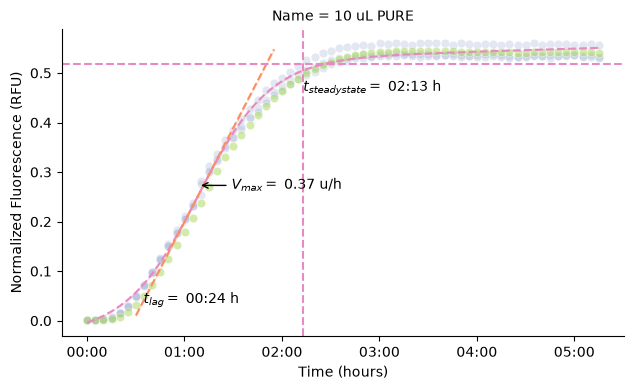
Figure 1:Example reactions (10 L PURE in triplicate at a typical composition) fit to a logistic curve with linear drift. Dots represent fluorescence at each timepoint (individual replicates in blue, mean of replicates in green). Time-to-completion (), lag time (), and maximum reaction rate () are plotted as well. Vertical and horizontal dashed red lines represent time-to-completion and drift corrected steady state fluorescence (), respectively. Orange dashed line represents the tangent line at the inflection point. The slope of this line is and the x-intercept of this line is . The fitted curve is plotted as a red dashed curve on top of data points.
In addition to the above fit parameters, we also report three derived parameters that summarize useful features of the curve:
Maximum reaction rate (): the maximum slope of the sigmoid, which occurs at and equals . This is not the Michaelis–Menten . Use for downstream calculations that require a slope with units (). When comparing reaction rates across conditions, use instead.
Lag time (): the time it takes for the reaction to “start” (units of ). Explicitly, the x-intercept of the line tangent to the inflection point () on the sigmoid. This is metric is related to transcription lag time, translation lag time, and the maturation time of your reporter.
Time-to-completion (): the time at which the reaction is “finished” (units of ). Explicitly, when the sigmoid reaches a chosen fraction of its asymptote (default ). can be derived analytically from the model as
Drift is intentionally excluded from this calculation; we believe excluding it gives us more accurate estimates of when the reaction finished.
How to use the CDK to model your reactions
This primer assumes you already have:
data from an experiment in a format that the CDK can handle (see
cdk.instrument.platereaderfor details),a platemap that describes what’s in each well of your experiment (see our note on using platemaps),
(optional) a fluorescent standard on the plate that you can use to normalize your data.
You can use the platereader module of the CDK to load platereader data and plot kinetic fits. Here’s a code snippet example:
from cdk.analysis.cytosol import platereader as pr

data = pr.load_platereader_data(
    path="path-to-timecourse-data.txt",
    platemap="path-to-platemap.csv",
)

graph, kinetics_df = pr.plot_kinetics(
    data,
    fit_function_name="sigmoid_drift"
)
This code snippet produces the following per group of conditions:
plots of raw traces with the fitted model overlaid
a summary plot of , , , and [JB: do you have to call
plot_summary()to get this?]a tidy DataFrame of the fit parameters (here,
kinetics_df)
The CDK currently defaults to fit_function_name="sigmoid_drift". If you don’t want to model drift, replace "sigmoid_drift" with "sigmoid".
We’ve included an example jupyter notebook titled “Kinetics Analysis Tutorial” with more examples of CDK usage using a simple dataset.
Common pitfalls and limitations
Truncated reactions. If your reaction isn’t finished by the last time point in your experiment, the CDK will cheerfully return a poor fit with small residuals. This is a known bug and we are working on building automated checks for this. CHECK YOUR FITS by visually inspecting if the curve reaches steady state and how well the fit matches the curve.
Reporting results without normalization. Before normalization, your data is in your plate reader’s native fluorescence units (arbitrary). For comparisons within the same experimental run, this is acceptable, however these data will not be comparable to other experiments. You should normalize your fluorescences to a known, calibrated fluorescent standard.
Sigmoid doesn’t describe your data. The sigmoid fit is good at summarizing a simple, “well-behaved” trace in four numbers, but has drawbacks. Specifically, it cannot represent:
asymmetric rise/fall (use Gompertz or a generalized sigmoid),
a biphasic reaction, e.g., when a module starts working later in a run (ClpXP-mediated degradation catching up to production),
explicit resource-exhaustion dynamics (better captured by a mechanistic model).
- CDK
- cell development kit