


20251208 Analysis (Group 1)
Analyze time-series fluorescence data from PURE (Protein synthesis Using Recombinant Elements) experiments.
20251208 Analysis (Group 1)
Setup
%load_ext autoreload
%autoreload 2

import pandas as pd
import seaborn as sns
import matplotlib.pyplot as plt

# Import the cdk platereader module
from cdk.analysis.cytosol import platereader as pr

# Set up plotting
pr.plot_setup()
Load Data
# Specify file paths
data_file = "./platereader/20251208-134617-cytation5-pure-timecourse-gfp--biotek-cdk.txt"
platemap_file = "platemap-G1.csv"

# Load data
data, platemap = pr.load_platereader_data(
    data_file=data_file,
    platemap_file=platemap_file,
    platereader="biotek-cdk"  # Options: "cytation", "envision", "biotek-cdk"
)

# Checkout first few rows
data.head()Plot Raw Curves
g = pr.plot_curves(data=data)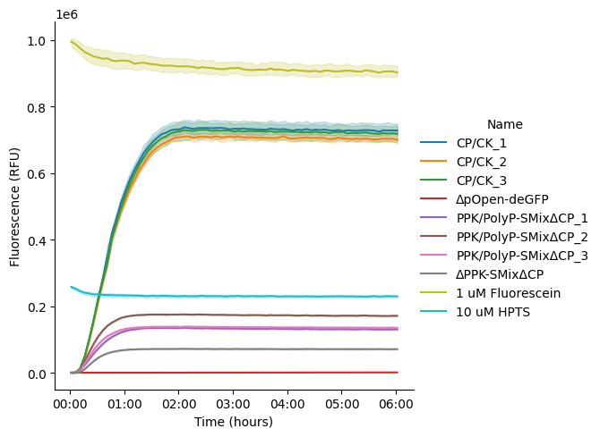
Normalize Data
data = pr.normalize_data_to_controls(data, ctrl_name = '1 uM Fluorescein')Data Normalized to 1 uM Fluorescein in col data_normalized. The active column for subsequent operations is: data_normalized
Now replot your curves to see them normalized
g = pr.plot_curves(data=data)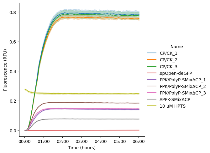
replace_dict = {'ΔPPK-SMixΔCP':'-PPK Negative Control',
                'ΔpOpen-deGFP':'-DNA Negative Control',
                'PPK/PolyP-SMixΔCP_1': 'PolyP/PPK_1',
                'PPK/PolyP-SMixΔCP_2': 'PolyP/PPK_2',
                'PPK/PolyP-SMixΔCP_3': 'PolyP/PPK_3'
               }

custom_order = ['CP/CK_1',
                'CP/CK_2',
                'CP/CK_3',
                'PolyP/PPK_1',
                'PolyP/PPK_2',
                'PolyP/PPK_3',
                '-PPK Negative Control',
                '-DNA Negative Control']

color_dict = {
    'CP/CK_1': '#1f77b4',      # Dark blue
    'CP/CK_2': '#4fa3d1',      # Medium blue
    'CP/CK_3': '#87ceeb',      # Light blue
    'PolyP/PPK_1': '#d62728',  # Dark red
    'PolyP/PPK_2': '#ff6b6b',  # Medium red
    'PolyP/PPK_3': '#ff9999',  # Light red
    '-PPK Negative Control': '#9467bd',  # Purple
    '-DNA Negative Control': '#000000'   # Black
}

data_rename = data
data_rename['Name'] = data['Name'].replace(replace_dict)
p = pr.plot_curves(data_rename[data_rename["Sample Type"] != "Standard"],
                   hue_order=custom_order,
                   palette=color_dict)
p.set(ylim=(0, 1.1))
plt.savefig("kinetics-group1.png")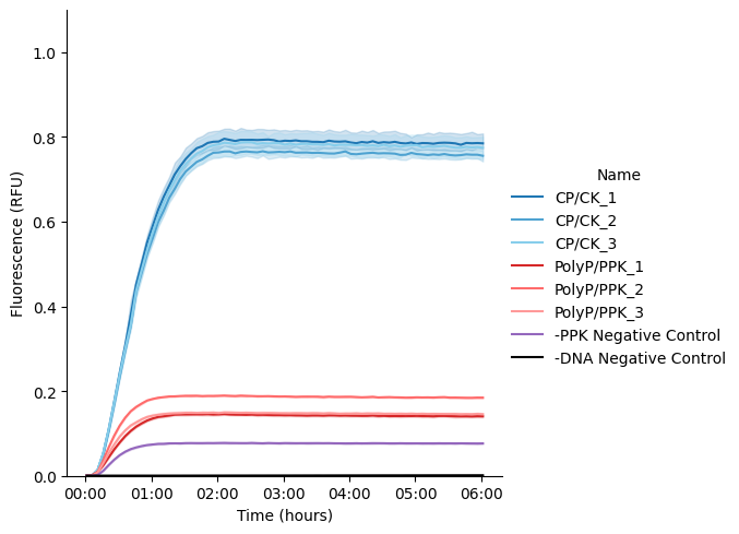
Kinetic Analysis
Metrics extracted:
Vmax (
Velocity Max): Maximum rate of fluorescence increase (slope at inflection point)Lag time: Time to reach the exponential phase
Steady-state: Final fluorescence level and time to reach 95% of asymptote
Drift: Rate of signal decay or increase after steady-state
R²: Goodness of fit
# Perform kinetic analysis using sigmoid_drift model
kinetics = pr.kinetic_analysis(
    data=data,
    group_by=['Name'],  # Group by experimental condition
)

kinetics.head()
PROVIDING AVERAGED KINETICS
Visualize Fits on Individual Wells
# Plot kinetic fits
g, kinetics = pr.plot_kinetics(data, kinetics=kinetics, group_by=["Name"])
plt.savefig("kinetic-fits-group1.png")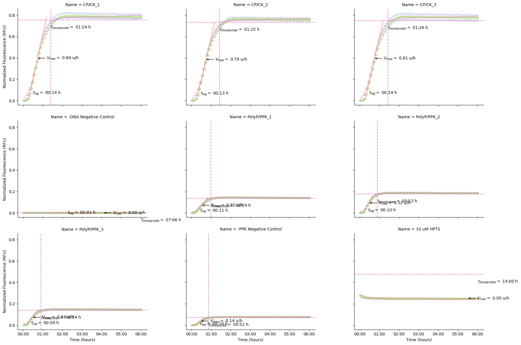
pr.kinetic_analysis_summary(data)PROVIDING AVERAGED KINETICS
Summary Plots
pr.plot_summary(data[data["Sample Type"] == "Sample"], show_plot=False)
plt.savefig("kinetics-summary-1.png")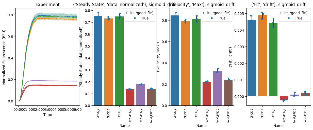
Key Metrics Explained
1. Steady-State Level (Steady State, Data)
The final fluorescence value reached by the reaction
Represents the total amount of protein produced
Higher values indicate greater expression yield
2. Maximum Velocity (Velocity, Max)
The steepest slope of the fluorescence curve (at the inflection point)
Units: RFU per second
Reflects the peak rate of protein synthesis
Sensitive to enzyme activity, substrate availability, and reaction conditions
3. Lag Time (Lag, Time)
Time before exponential fluorescence increase begins
May reflect time for ribosome assembly or initial translation steps
Shorter lag times suggest faster reaction initiation
4. Drift (Fit, drift)
Rate of fluorescence change after reaching steady-state
Positive drift: continued synthesis or aggregation
Negative drift: photobleaching, protein degradation, or quenching
Units: RFU per second
5. R² Value (Fit, R^2)
Goodness of fit (0 to 1, higher is better)
R² > 0.98 indicates excellent fit
Poor fits may indicate noisy data, overflow errors, or non-sigmoid kinetics
Tips and Troubleshooting
Overflow errors: Wells with
OVRFLWorNaNvalues are automatically excluded from fittingPoor fits (low R²): Inspect raw curves for anomalies (bubbles, evaporation, pipetting errors)
Drift: Sometimes seen in kinetics curves; use
sigmoid_driftmodelMultiple replicates: Always include technical replicates and report error bars
Comparing conditions: Normalize or blank data consistently across all samples
Next Steps
Export kinetics results:
pr.export_kinetics(kinetics, 'results.csv')Statistical analysis: Use
scipy.statsorstatsmodelsfor ANOVA/t-testsParameter optimization: Vary Mg²⁺, K⁺, or other conditions to maximize Vmax or steady-state
Mechanistic modeling: Fit ODE models to extract biological rate constants