

!pip install nucleus-cdk==0.5.0rc2 | tail -n2

# Surface a failed install here, rather than as a confusing ModuleNotFoundError
# in the import cell below.
import importlib.metadata as md
assert md.version("nucleus-cdk") == "0.5.0rc2", f"got {md.version('nucleus-cdk')}"
Requirement already satisfied: urllib3<3,>=1.21.1 in /opt/homebrew/Caskroom/miniforge/base/lib/python3.12/site-packages (from requests->panel>=1.0->hvplot<0.12.0,>=0.11.1->nucleus-cdk==0.5.0rc2) (2.5.0)
Requirement already satisfied: certifi>=2017.4.17 in /opt/homebrew/Caskroom/miniforge/base/lib/python3.12/site-packages (from requests->panel>=1.0->hvplot<0.12.0,>=0.11.1->nucleus-cdk==0.5.0rc2) (2025.11.12)
import pandas as pd
import matplotlib.pyplot as plt
import seaborn as sns

from cdk.analysis.cytosol import platereader as pr
# import platereader as pr
# Initialize plotting
pr.plot_setup()
import sys# !ls bnext/experiments/20251106_labcraft_protein_sweep_01data = pr.load_platereader_data("data/20251106-191540-cytation5-pure-timecourse-gfp-labcraft-protein-sweep1-biotek-cdk.txt")
platemap = pd.read_csv("data/concentration_key.csv")
# platemap.columns = ["Well", "Mg (mM)", "Ribo (uM)", "T7 (ng/ul)", "Water"]
# platemap["Name"] = "GFP " + platemap["[DNA] (nM)"].astype(str) + " nM"
platemap.rename(columns={'Well ID':"Well"}, inplace=True)
platemap = platemap.fillna(0)
# platemap.columns
sweep_cols= ['Mg_mM', 'Ribo_uM', 'T7poly_ng/ul']
for values, g in platemap.groupby(sweep_cols):
mg, ribo, T7 = values
name = f"Mg {mg}; R {ribo}; T7 {T7}"
platemap.loc[g.index, "Name"] = name
platemap
data = data.merge(platemap)platemap.head()
data.head()Loading...
dataLoading...
pr.plot_curves(data)<seaborn.axisgrid.FacetGrid at 0x111912f00>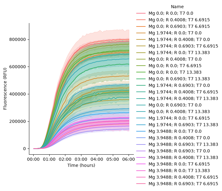
# pr.plot_curves(data, hue=sweep_cols[0], col=sweep_cols[2], palette="viridis")
print(sweep_cols)
['Mg_mM', 'Ribo_uM', 'T7poly_ng/ul']
sns.relplot(data, x="Time", y="Data", row=sweep_cols[0], col=sweep_cols[2], hue=sweep_cols[1], kind="line") #, hue="Name")<seaborn.axisgrid.FacetGrid at 0x111bdaa50>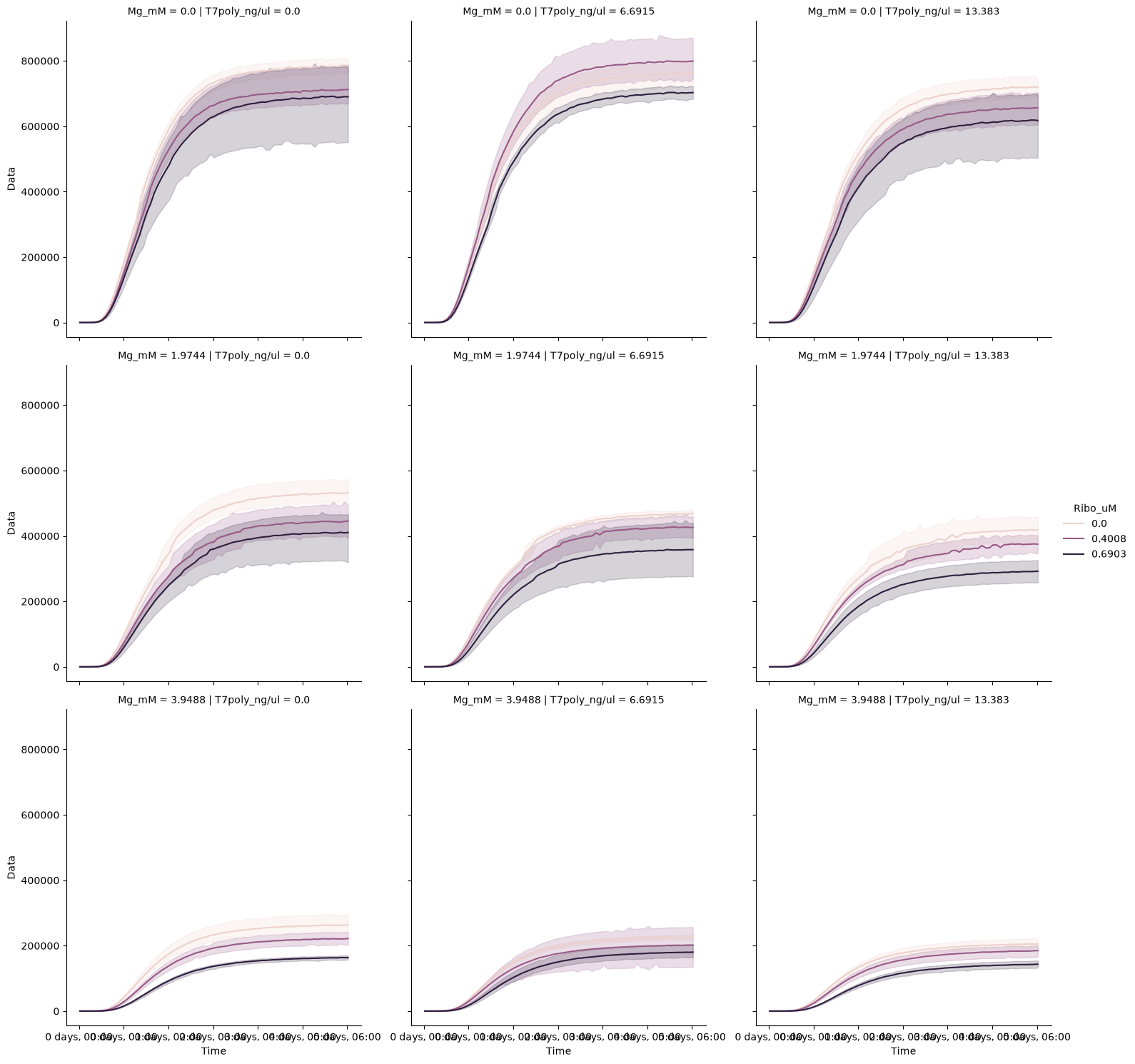
kinetics = pr.kinetic_analysis(data, group_by=["Name"])
kinetics
/private/tmp/claude-501/-Users-sharonnewman-Documents-general-nucleus-skills/4a8d6065-9e0a-4e14-b326-0bffb6d3273b/scratchpad/cdkenv/lib/python3.12/site-packages/pandas/core/arraylike.py:399: RuntimeWarning: overflow encountered in exp
result = getattr(ufunc, method)(*inputs, **kwargs)
/private/tmp/claude-501/-Users-sharonnewman-Documents-general-nucleus-skills/4a8d6065-9e0a-4e14-b326-0bffb6d3273b/scratchpad/cdkenv/lib/python3.12/site-packages/pandas/core/arraylike.py:399: RuntimeWarning: overflow encountered in exp
  result = getattr(ufunc, method)(*inputs, **kwargs)
/private/tmp/claude-501/-Users-sharonnewman-Documents-general-nucleus-skills/4a8d6065-9e0a-4e14-b326-0bffb6d3273b/scratchpad/cdkenv/lib/python3.12/site-packages/pandas/core/arraylike.py:399: RuntimeWarning: overflow encountered in exp
  result = getattr(ufunc, method)(*inputs, **kwargs)
PROVIDING AVERAGED KINETICS
Loading...
kinetics.columns
ss = kinetics["Steady State"]["Data"].reset_index().merge(platemap)
# ss = kinetics["Velocity"]["Max"].reset_index().merge(platemap)
# data_name = 'Max' #Data
data_name = 'Data'pr.plot_kinetics(data, group_by=["Name"])/private/tmp/claude-501/-Users-sharonnewman-Documents-general-nucleus-skills/4a8d6065-9e0a-4e14-b326-0bffb6d3273b/scratchpad/cdkenv/lib/python3.12/site-packages/pandas/core/arraylike.py:399: RuntimeWarning: overflow encountered in exp
result = getattr(ufunc, method)(*inputs, **kwargs)
/private/tmp/claude-501/-Users-sharonnewman-Documents-general-nucleus-skills/4a8d6065-9e0a-4e14-b326-0bffb6d3273b/scratchpad/cdkenv/lib/python3.12/site-packages/pandas/core/arraylike.py:399: RuntimeWarning: overflow encountered in exp
  result = getattr(ufunc, method)(*inputs, **kwargs)
/private/tmp/claude-501/-Users-sharonnewman-Documents-general-nucleus-skills/4a8d6065-9e0a-4e14-b326-0bffb6d3273b/scratchpad/cdkenv/lib/python3.12/site-packages/pandas/core/arraylike.py:399: RuntimeWarning: overflow encountered in exp
  result = getattr(ufunc, method)(*inputs, **kwargs)
PROVIDING AVERAGED KINETICS
(<seaborn.axisgrid.FacetGrid at 0x112f36f00>,
                                                 Velocity                      \
                                                     Time      Data       Max
 Name
 Mg 0.0; R 0.0; T7 0.0          0 days 01:25:06.384157767 391036.93 464495.78
 Mg 0.0; R 0.0; T7 13.383       0 days 01:23:12.227808558 357873.19 379802.81
 Mg 0.0; R 0.0; T7 6.6915       0 days 01:23:00.991286042 367973.45 427639.32
 Mg 0.0; R 0.4008; T7 0.0       0 days 01:24:07.313832339 356736.31 414825.70
 Mg 0.0; R 0.4008; T7 13.383    0 days 01:25:42.038596308 330913.22 334829.87
 Mg 0.0; R 0.4008; T7 6.6915    0 days 01:23:42.845952033 392106.89 449012.30
 Mg 0.0; R 0.6903; T7 0.0       0 days 01:29:55.710262378 340358.30 372208.22
 Mg 0.0; R 0.6903; T7 13.383    0 days 01:30:56.793676442 310808.77 303268.05
 Mg 0.0; R 0.6903; T7 6.6915    0 days 01:26:35.570398910 355678.24 362781.19
 Mg 1.9744; R 0.0; T7 0.0       0 days 01:31:10.047957710 266026.68 265537.28
 Mg 1.9744; R 0.0; T7 13.383    0 days 01:22:38.831052047 209776.90 181448.51
 Mg 1.9744; R 0.0; T7 6.6915    0 days 01:29:22.965593733 234582.15 223475.76
 Mg 1.9744; R 0.4008; T7 0.0    0 days 01:32:26.433102526 223002.30 199158.18
 Mg 1.9744; R 0.4008; T7 13.383 0 days 01:24:06.960227581 188265.56 158092.24
 Mg 1.9744; R 0.4008; T7 6.6915 0 days 01:29:32.494454971 214017.22 191450.93
 Mg 1.9744; R 0.6903; T7 0.0    0 days 01:37:11.559421711 205806.38 185203.77
 Mg 1.9744; R 0.6903; T7 13.383 0 days 01:33:27.475317193 146055.89 134875.18
 Mg 1.9744; R 0.6903; T7 6.6915 0 days 01:35:55.723313741 179588.56 163286.65
 Mg 3.9488; R 0.0; T7 0.0       0 days 01:30:38.899218105 131767.15 129933.86
 Mg 3.9488; R 0.0; T7 13.383    0 days 01:29:35.896920936 102768.54  96198.01
 Mg 3.9488; R 0.0; T7 6.6915    0 days 01:29:18.900008816 113198.80 109991.03
 Mg 3.9488; R 0.4008; T7 0.0    0 days 01:36:19.162132231 110818.63 104481.71
 Mg 3.9488; R 0.4008; T7 13.383 0 days 01:34:15.104488488  92453.17  81578.59
 Mg 3.9488; R 0.4008; T7 6.6915 0 days 01:30:49.317234001 100944.78  96721.92
 Mg 3.9488; R 0.6903; T7 0.0    0 days 01:44:19.124703433  81955.51  71528.78
 Mg 3.9488; R 0.6903; T7 13.383 0 days 01:45:24.189728286  67605.95  59776.16
 Mg 3.9488; R 0.6903; T7 6.6915 0 days 01:42:58.014040578  90240.65  78414.00

                                                      Lag            \
                                                     Time      Data
 Name
 Mg 0.0; R 0.0; T7 0.0          0 days 00:34:29.416211466  58273.39
 Mg 0.0; R 0.0; T7 13.383       0 days 00:26:26.200437412  15446.97
 Mg 0.0; R 0.0; T7 6.6915       0 days 00:31:07.936658955  36882.12
 Mg 0.0; R 0.4008; T7 0.0       0 days 00:32:35.902041874  30788.26
 Mg 0.0; R 0.4008; T7 13.383    0 days 00:26:29.008152804  11516.61
 Mg 0.0; R 0.4008; T7 6.6915    0 days 00:31:18.592564633  33526.11
 Mg 0.0; R 0.6903; T7 0.0       0 days 00:34:46.926552948  42570.22
 Mg 0.0; R 0.6903; T7 13.383    0 days 00:29:02.185712247  12702.54
 Mg 0.0; R 0.6903; T7 6.6915    0 days 00:27:44.533647051  15200.72
 Mg 1.9744; R 0.0; T7 0.0       0 days 00:30:54.371716438  18549.69
 Mg 1.9744; R 0.0; T7 13.383    0 days 00:12:12.048795450 -13817.18
 Mg 1.9744; R 0.0; T7 6.6915    0 days 00:26:20.096878108  10803.28
 Mg 1.9744; R 0.4008; T7 0.0    0 days 00:24:19.111957006   5599.48
 Mg 1.9744; R 0.4008; T7 13.383 0 days 00:12:14.443602857 -15926.72
 Mg 1.9744; R 0.4008; T7 6.6915 0 days 00:21:36.523796879   1314.50
 Mg 1.9744; R 0.6903; T7 0.0    0 days 00:30:38.184571957  10962.55
 Mg 1.9744; R 0.6903; T7 13.383 0 days 00:28:23.405745736   3120.04
 Mg 1.9744; R 0.6903; T7 6.6915 0 days 00:30:22.672605073   8290.13
 Mg 3.9488; R 0.0; T7 0.0       0 days 00:29:43.509092187   5846.39
 Mg 3.9488; R 0.0; T7 13.383    0 days 00:25:27.577661245   1195.47
 Mg 3.9488; R 0.0; T7 6.6915    0 days 00:27:33.175679690   2978.65
 Mg 3.9488; R 0.4008; T7 0.0    0 days 00:32:40.159888568   5575.75
 Mg 3.9488; R 0.4008; T7 13.383 0 days 00:26:11.535109176    645.93
 Mg 3.9488; R 0.4008; T7 6.6915 0 days 00:29:05.448459917   3539.95
 Mg 3.9488; R 0.6903; T7 0.0    0 days 00:35:33.186861893   4052.33
 Mg 3.9488; R 0.6903; T7 13.383 0 days 00:36:49.789627331   4270.67
 Mg 3.9488; R 0.6903; T7 6.6915 0 days 00:33:44.857105481   3507.00

                                             Steady State            \
                                                     Time      Data
 Name
 Mg 0.0; R 0.0; T7 0.0          0 days 02:39:37.467556420 742970.17
 Mg 0.0; R 0.0; T7 13.383       0 days 02:46:46.647685590 679959.06
 Mg 0.0; R 0.0; T7 6.6915       0 days 02:39:24.090979379 699149.56
 Mg 0.0; R 0.4008; T7 0.0       0 days 02:39:58.550519721 677798.99
 Mg 0.0; R 0.4008; T7 13.383    0 days 02:52:52.879261863 628735.13
 Mg 0.0; R 0.4008; T7 6.6915    0 days 02:40:51.877068735 745003.09
 Mg 0.0; R 0.6903; T7 0.0       0 days 02:51:06.966125290 646680.76
 Mg 0.0; R 0.6903; T7 13.383    0 days 03:02:05.511916839 590536.67
 Mg 0.0; R 0.6903; T7 6.6915    0 days 02:53:14.031522829 675788.65
 Mg 1.9744; R 0.0; T7 0.0       0 days 02:59:53.116987456 505450.70
 Mg 1.9744; R 0.0; T7 13.383    0 days 03:06:21.582267995 398576.11
 Mg 1.9744; R 0.0; T7 6.6915    0 days 03:02:12.178642696 445706.08
 Mg 1.9744; R 0.4008; T7 0.0    0 days 03:12:43.866952370 423704.36
 Mg 1.9744; R 0.4008; T7 13.383 0 days 03:09:55.931251162 357704.57
 Mg 1.9744; R 0.4008; T7 6.6915 0 days 03:09:33.217896087 406632.71
 Mg 1.9744; R 0.6903; T7 0.0    0 days 03:15:10.683704419 391032.12
 Mg 1.9744; R 0.6903; T7 13.383 0 days 03:09:15.122628326 277506.19
 Mg 1.9744; R 0.6903; T7 6.6915 0 days 03:12:26.037219836 341218.27
 Mg 3.9488; R 0.0; T7 0.0       0 days 03:00:20.435802617 250357.58
 Mg 3.9488; R 0.0; T7 13.383    0 days 03:04:01.467536549 195260.22
 Mg 3.9488; R 0.0; T7 6.6915    0 days 03:00:14.539588342 215077.72
 Mg 3.9488; R 0.4008; T7 0.0    0 days 03:10:01.571665405 210555.39
 Mg 3.9488; R 0.4008; T7 13.383 0 days 03:14:27.014915055 175661.01
 Mg 3.9488; R 0.4008; T7 6.6915 0 days 03:01:42.225029697 191795.09
 Mg 3.9488; R 0.6903; T7 0.0    0 days 03:25:33.410805916 155715.47
 Mg 3.9488; R 0.6903; T7 13.383 0 days 03:26:21.489744063 128451.30
 Mg 3.9488; R 0.6903; T7 6.6915 0 days 03:24:52.372623242 171457.24

                                                                               Fit  \
                                                                            params
 Name
 Mg 0.0; R 0.0; T7 0.0           [782073.8658722346, 2.375343636306762, 1.41844...
 Mg 0.0; R 0.0; T7 13.383        [715746.3803741209, 2.120389798812113, 1.38672...
 Mg 0.0; R 0.0; T7 6.6915        [735946.9077719614, 2.3319712416741716, 1.3836...
 Mg 0.0; R 0.4008; T7 0.0        [713472.616785697, 2.3321619476225703, 1.40203...
 Mg 0.0; R 0.4008; T7 13.383     [661826.4497586022, 2.0279097397860024, 1.4283...
 Mg 0.0; R 0.4008; T7 6.6915     [784213.7776576624, 2.2903019405603517, 1.3952...
 Mg 0.0; R 0.6903; T7 0.0        [680716.5903602357, 2.1819654470998326, 1.4988...
 Mg 0.0; R 0.6903; T7 13.383     [621617.5452810051, 1.9409725828795965, 1.5157...
 Mg 0.0; R 0.6903; T7 6.6915     [711356.4727441198, 2.040622517734187, 1.44321...
 Mg 1.9744; R 0.0; T7 0.0        [532053.3699681616, 1.9927951351190756, 1.5194...
 Mg 1.9744; R 0.0; T7 13.383     [419553.79744963074, 1.7154597418411308, 1.377...
 Mg 1.9744; R 0.0; T7 6.6915     [469164.29909062316, 1.9047340489697548, 1.489...
 Mg 1.9744; R 0.4008; T7 0.0     [446004.59312138916, 1.771045129517986, 1.5406...
 Mg 1.9744; R 0.4008; T7 13.383  [376531.1269253074, 1.6864992087448423, 1.4019...
 Mg 1.9744; R 0.4008; T7 6.6915  [428034.43628156517, 1.7775177326789922, 1.492...
 Mg 1.9744; R 0.6903; T7 0.0     [411612.76288470003, 1.806767669866755, 1.6198...
 Mg 1.9744; R 0.6903; T7 13.383  [292111.7806860807, 1.8444842465236158, 1.5576...
 Mg 1.9744; R 0.6903; T7 6.6915  [359177.12895069976, 1.8344457780391827, 1.598...
 Mg 3.9488; R 0.0; T7 0.0        [263534.2964317678, 1.9699816019059575, 1.5108...
 Mg 3.9488; R 0.0; T7 13.383     [205537.07077621744, 1.8715553549498225, 1.493...
 Mg 3.9488; R 0.0; T7 6.6915     [226397.5952397759, 1.9429951601790996, 1.4885...
 Mg 3.9488; R 0.4008; T7 0.0     [221637.2520672017, 1.8856147009081166, 1.6053...
 Mg 3.9488; R 0.4008; T7 13.383  [184906.33117008847, 1.76332935318427, 1.57086...
 Mg 3.9488; R 0.4008; T7 6.6915  [201889.56427534568, 1.9547755507089732, 1.513...
 Mg 3.9488; R 0.6903; T7 0.0     [163911.01667216455, 1.7452474371207776, 1.738...
 Mg 3.9488; R 0.6903; T7 13.383  [135211.8970598355, 1.78584639750524, 1.756719...
 Mg 3.9488; R 0.6903; T7 6.6915  [180481.3096179662, 1.7345681546538323, 1.7161...


                                 R^2    drift
 Name
 Mg 0.0; R 0.0; T7 0.0          1.00  5986.48
 Mg 0.0; R 0.0; T7 13.383       1.00 14517.91
 Mg 0.0; R 0.0; T7 6.6915       1.00 15055.08
 Mg 0.0; R 0.4008; T7 0.0       1.00 10248.63
 Mg 0.0; R 0.4008; T7 13.383    1.00 12056.37
 Mg 0.0; R 0.4008; T7 6.6915    1.00 15223.10
 Mg 0.0; R 0.6903; T7 0.0       1.00  8830.31
 Mg 0.0; R 0.6903; T7 13.383    1.00 11147.12
 Mg 0.0; R 0.6903; T7 6.6915    1.00 12554.64
 Mg 1.9744; R 0.0; T7 0.0       1.00  8533.08
 Mg 1.9744; R 0.0; T7 13.383    1.00 11364.84
 Mg 1.9744; R 0.0; T7 6.6915    1.00  8501.90
 Mg 1.9744; R 0.4008; T7 0.0    1.00  9000.57
 Mg 1.9744; R 0.4008; T7 13.383 0.99 10684.48
 Mg 1.9744; R 0.4008; T7 6.6915 1.00  9345.35
 Mg 1.9744; R 0.6903; T7 0.0    1.00  7248.21
 Mg 1.9744; R 0.6903; T7 13.383 1.00  5711.82
 Mg 1.9744; R 0.6903; T7 6.6915 1.00  6520.42
 Mg 3.9488; R 0.0; T7 0.0       1.00  4652.97
 Mg 3.9488; R 0.0; T7 13.383    1.00  4166.14
 Mg 3.9488; R 0.0; T7 6.6915    1.00  4317.58
 Mg 3.9488; R 0.4008; T7 0.0    1.00  3817.49
 Mg 3.9488; R 0.4008; T7 13.383 1.00  3832.44
 Mg 3.9488; R 0.4008; T7 6.6915 1.00  3729.18
 Mg 3.9488; R 0.6903; T7 0.0    1.00  2851.99
 Mg 3.9488; R 0.6903; T7 13.383 1.00  3883.35
 Mg 3.9488; R 0.6903; T7 6.6915 1.00  3297.77  )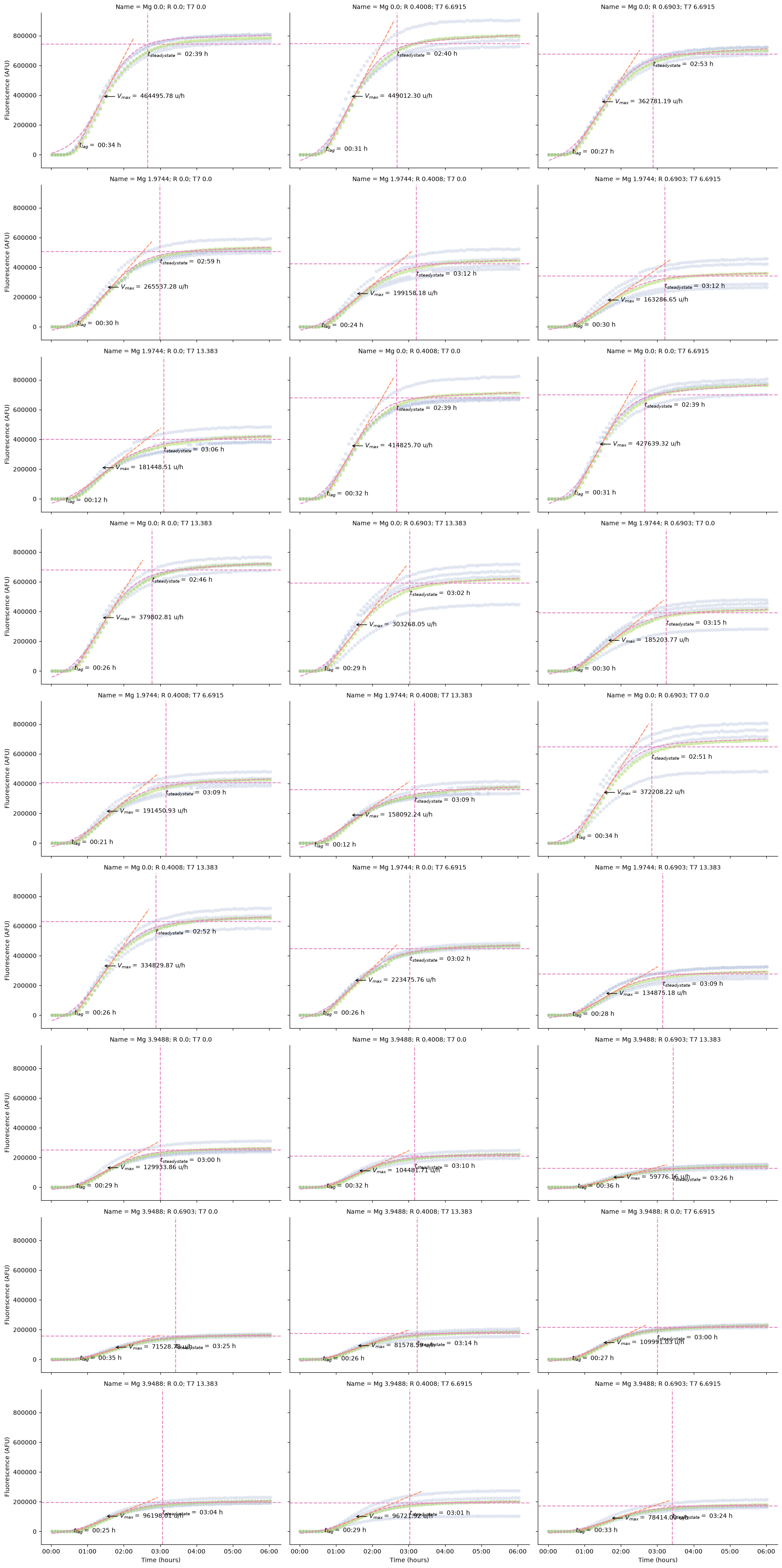
ss.head()Loading...
ss.to_csv('steady_states.csv', index=False)df = ss
# Average replicates
means = df.groupby(['Mg_mM', 'Ribo_uM', 'T7poly_ng/ul'], as_index=False)[data_name].mean()
# Global min/max for shared color bar
data_min = means[data_name].min()
data_max = means[data_name].max()
t7_values = means['Mg_mM'].unique()
n_plots = len(t7_values)
fig, axes = plt.subplots(1, n_plots, figsize=(7*n_plots, 6), squeeze=False)
for idx, t7 in enumerate(sorted(t7_values)):
slice_df = means[means['Mg_mM'] == t7]
pivot = slice_df.pivot(index='Ribo_uM', columns='T7poly_ng/ul', values=data_name)
ax = axes[0, idx]
hm = sns.heatmap(
pivot, annot=True, cmap='viridis',
vmin=data_min, vmax=data_max, # shared color scale
cbar=idx==n_plots-1, cbar_ax=None if idx < n_plots-1 else plt.gcf().add_axes([0.93, 0.3, 0.02, 0.4]),
ax=ax
)
ax.set_title(f'Mg_mM={t7}')
ax.set_xlabel('T7poly_ng/ul')
ax.set_ylabel('Ribo_uM')
plt.suptitle("Vmax")
plt.tight_layout(rect=[0, 0, 0.9, 1]) # Leave space for color bar
plt.show()/var/folders/4l/5bp8d9ks6v15tkhzpbszxxpc0000gn/T/ipykernel_21493/806804362.py:29: UserWarning: This figure includes Axes that are not compatible with tight_layout, so results might be incorrect.
plt.tight_layout(rect=[0, 0, 0.9, 1]) # Leave space for color bar
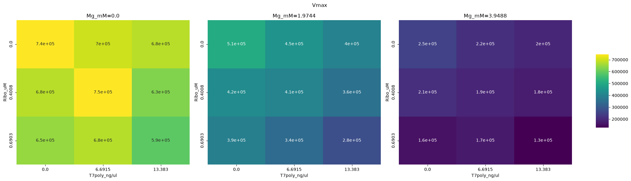
df = ss
# Average replicates
means = df.groupby(['Mg_mM', 'Ribo_uM', 'T7poly_ng/ul'], as_index=False)[data_name].mean()

# Global min/max for shared color bar
data_min = means[data_name].min()
data_max = means[data_name].max()

t7_values = means['T7poly_ng/ul'].unique()
n_plots = len(t7_values)
fig, axes = plt.subplots(1, n_plots, figsize=(7*n_plots, 6), squeeze=False)

for idx, t7 in enumerate(sorted(t7_values)):
    slice_df = means[means['T7poly_ng/ul'] == t7]
    pivot = slice_df.pivot(index='Ribo_uM', columns='Mg_mM', values=data_name)
    ax = axes[0, idx]
    hm = sns.heatmap(
        pivot, annot=True, cmap='viridis',
        vmin=data_min, vmax=data_max,  # shared color scale
        cbar=idx==n_plots-1, cbar_ax=None if idx < n_plots-1 else plt.gcf().add_axes([0.93, 0.3, 0.02, 0.4]),
        ax=ax
    )
    ax.set_title(f'T7poly_ng/ul={t7}')
    ax.set_xlabel('Mg_mM')
    ax.set_ylabel('Ribo_uM')

plt.suptitle("Vmax")
plt.tight_layout(rect=[0, 0, 0.9, 1])  # Leave space for color bar
plt.show()
/var/folders/4l/5bp8d9ks6v15tkhzpbszxxpc0000gn/T/ipykernel_21493/2296589567.py:28: UserWarning: This figure includes Axes that are not compatible with tight_layout, so results might be incorrect.
plt.tight_layout(rect=[0, 0, 0.9, 1]) # Leave space for color bar
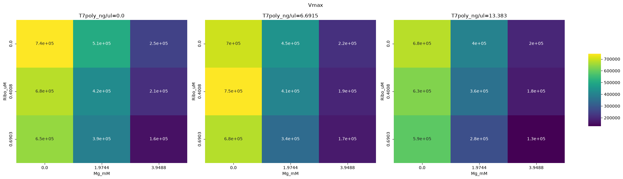
# data_name = 'Max' #Data
# Average replicates
means = df.groupby(['Mg_mM', 'Ribo_uM', 'T7poly_ng/ul'], as_index=False)[data_name].mean()

# 3D scatter/Surface for each unique T7poly_ng/ul, or all together using T7poly as color:
fig = plt.figure(figsize=(10, 7))
ax = fig.add_subplot(111, projection='3d')

# Normalize T7poly for color mapping
norm = plt.Normalize(means['T7poly_ng/ul'].min(), means['T7poly_ng/ul'].max())
colors = plt.cm.viridis(norm(means['T7poly_ng/ul']))

scat = ax.scatter(means['Mg_mM'], means['Ribo_uM'], means[data_name],
                  c=colors, s=60, edgecolor='k')

# Add colorbar for T7poly_ng/ul
mappable = plt.cm.ScalarMappable(cmap='viridis', norm=norm)
mappable.set_array(means['T7poly_ng/ul'])
fig.colorbar(mappable, ax=ax, label='T7poly_ng/ul')

ax.set_xlabel('Mg_mM')
ax.set_ylabel('Ribo_uM')
ax.set_zlabel('Steady State Value')
ax.set_title('Steady State as a Function of Mg, Ribo, and T7RNAP')

plt.tight_layout()
plt.show()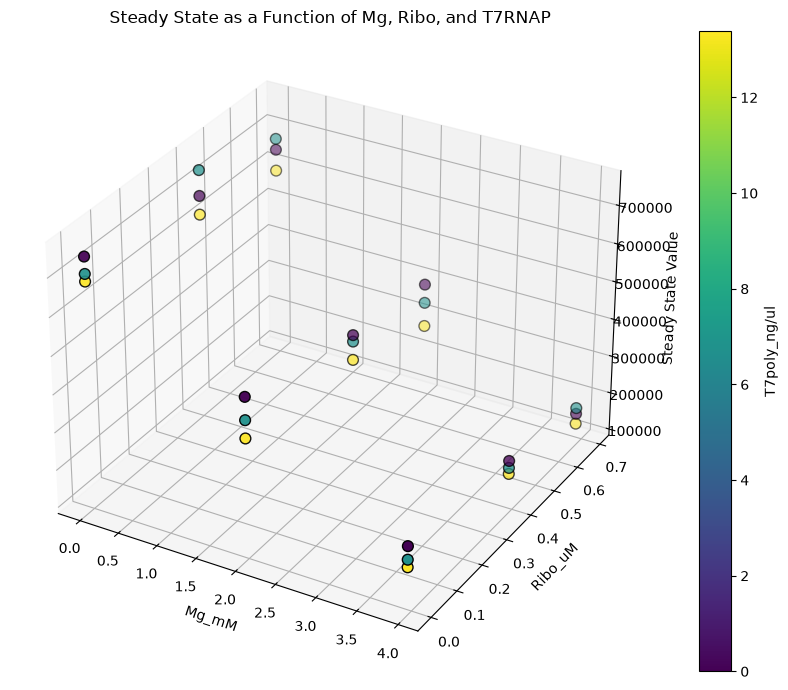
# Build a continuous palette for Ribo
norm = plt.Normalize(df['Ribo_uM'].min(), df['Ribo_uM'].max())
cmap = plt.cm.viridis

g = sns.relplot(
    data=df,
    x="Mg_mM", y="Data",
    col="T7poly_ng/ul", hue="Ribo_uM",  err_style='band', errorbar='sd',
    kind="line",
    facet_kws={'sharey': True, 'sharex': True},
    hue_norm=(df['Ribo_uM'].min(), df['Ribo_uM'].max())
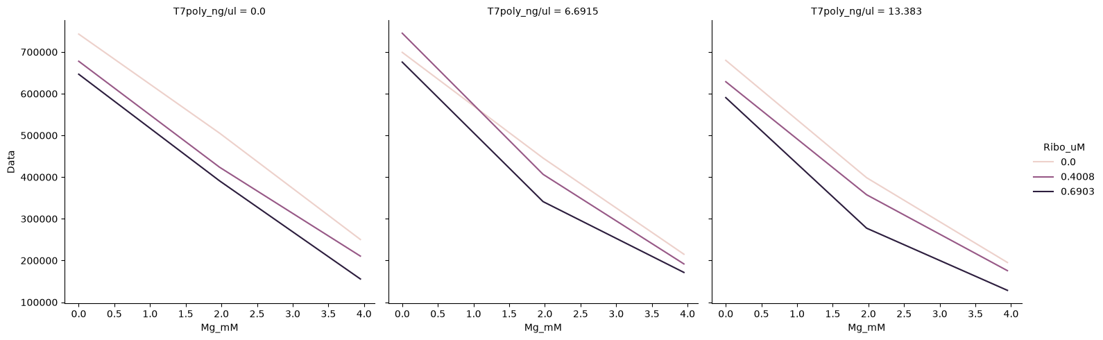
)
df.columnsIndex(['Name', 'Data', 'Well', 'Mg_mM', 'Ribo_uM', 'T7poly_ng/ul', 'Water_--'], dtype='object')def plot_main_effects(data, response_var):
# Get all columns except the response variable
factors = [col for col in data.columns if col != response_var]
# Plot each factor's main effect
for factor in factors:
plt.figure(figsize=(6, 4))
sns.pointplot(x=factor, y=response_var, data=data, errorbar="sd", markers="o", linestyles="-")
plt.title(f"Main Effect of {factor} on {response_var}")
plt.xlabel(factor)
plt.ylabel(response_var)
plt.show()
df["Steady State (AFU)"] = df["Data"]
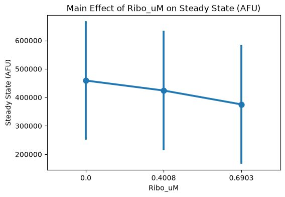
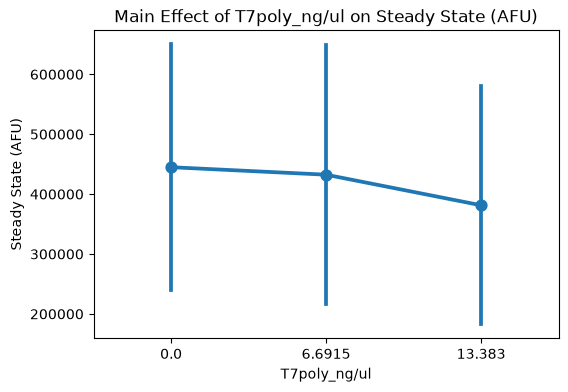
plot_main_effects(df[['Steady State (AFU)', 'Mg_mM', 'Ribo_uM', 'T7poly_ng/ul']], "Steady State (AFU)")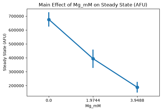
import math
def plot_main_effects(data, response_var):
    # Get all columns except the response variable
    factors = [col for col in data.columns if col != response_var]
    n = len(factors)

    # Determine subplot grid size
    cols = 3
    rows = math.ceil(n / cols)

    fig, axes = plt.subplots(rows, cols, figsize=(12, 4 * rows))
    axes = axes.flatten()  # flatten in case of 1 row

    for ax, factor in zip(axes, factors):
        sns.pointplot(
            x=factor,
            y=response_var,
            data=data,
            errorbar="sd",
            markers="o",
            linestyles="-",
            ax=ax
        )
        ax.set_title(f"Main Effect of {factor} on {response_var}")
        ax.set_xlabel(factor)
        ax.set_ylabel(response_var)

    # Hide any empty subplots
    for i in range(len(factors), len(axes)):
        axes[i].set_visible(False)

    plt.tight_layout()
    plt.show()

df["Steady State (AFU)"] = df["Data"]
plot_main_effects(df[['Steady State (AFU)', 'Mg_mM', 'Ribo_uM', 'T7poly_ng/ul']], "Steady State (AFU)")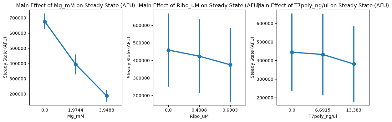
import numpy as np
from itertools import combinations
def plot_all_interactions(data, response_var):
    factors = [col for col in data.columns if col != response_var]
    factor_pairs = list(combinations(factors, 2))
    n = len(factor_pairs)

    cols = 3
    rows = math.ceil(n / cols)

    fig, axes = plt.subplots(rows, cols, figsize=(12, 5 * rows))
    axes = axes.flatten()

    for ax, (factor_x, factor_hue) in zip(axes, factor_pairs):

        levels = np.sort(data[factor_hue].unique())

        # Build a continuous colormap (viridis is great for continuous data)
        cmap = sns.color_palette("viridis", as_cmap=True)

        # Normalize hue values to [0,1] for colormap mapping
        if np.issubdtype(data[factor_hue].dtype, np.number):
            norm_levels = (levels - levels.min()) / (levels.max() - levels.min() + 1e-9)
        else:
            # For categorical: evenly spaced colors
            norm_levels = np.linspace(0, 1, len(levels))

        color_map = {level: cmap(norm) for level, norm in zip(levels, norm_levels)}

        # Plot per hue level
        for level in levels:
            subset = data[data[factor_hue] == level]

            # Scatter points
            sns.scatterplot(
                data=subset,
                x=factor_x,
                y=response_var,
                ax=ax,
                color=color_map[level],
                label=f"{factor_hue}: {level}"
            )

            # CI-smoothed line, same color
            sns.lineplot(
                data=subset,
                x=factor_x,
                y=response_var,
                ax=ax,
                color=color_map[level],
                errorbar="sd"
            )

        ax.set_title(f"Interaction: {factor_x} × {factor_hue}")
        ax.set_xlabel(factor_x)
        ax.set_ylabel(response_var)

    # Hide unused axes
    for i in range(len(factor_pairs), len(axes)):
        axes[i].set_visible(False)

    plt.tight_layout()
    plt.show()

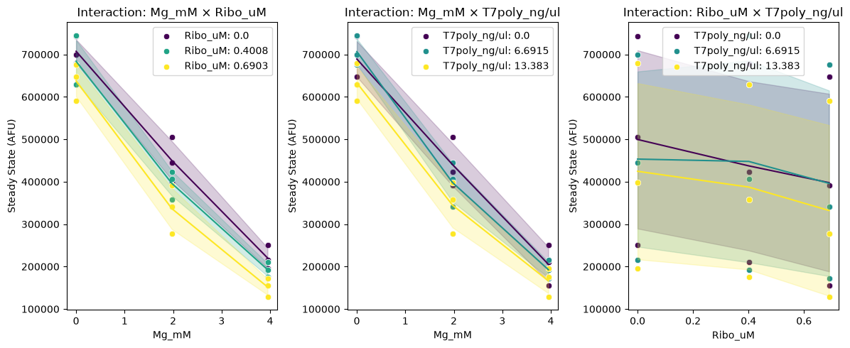
plot_all_interactions(df[['Steady State (AFU)', 'Mg_mM', 'Ribo_uM', 'T7poly_ng/ul']], "Steady State (AFU)")